Mortality rate models

Oct 11, 2026

Mortality rate models are mathematical functions that describe how the mortality rate changes with age: the rate at which people who have reached a given age die at that age. Everything else in a life table, from the share of people still alive at each birthday to life expectancy, follows from that one curve. The models are used to price annuities and life insurance, to smooth and extend life tables, to forecast population ageing, to compare the pace of ageing across species, and to test what an intervention against ageing actually changes.

The founding observation is the Gompertz law, published by the actuary Benjamin Gompertz in 1825: across adulthood, the mortality rate rises exponentially with age.¹ In people the rate doubles roughly every eight years,² so it grows two- to two-and-a-half-fold with each decade of adult life. Later models add terms for what the exponential misses: a constant that does not depend on age, added by William Makeham in 1860,³ and separate terms for the high mortality of infancy and the excess deaths of young adults.

Two questions run through the field. The first is whether the exponential rise continues to the end of life or slows into a mortality plateau at extreme ages. Plateaus are well documented in large laboratory cohorts of insects,⁴⁵ but in humans the evidence is contested, because a small rate of age-misreporting can manufacture a plateau.⁶⁷⁸ The second is why the mortality rate takes this shape at all. The shape also differs widely between species: in some animals and plants the mortality rate does not rise with age, or falls.⁹ A separate family of models, starting with Ronald Lee and Lawrence Carter’s in 1992, describes how the mortality rate at each age changes over calendar time; these are the standard tools of mortality forecasting.¹⁰

Terminology

A life table follows a group of people from birth, either a real generation or a hypothetical one, and records how many are still alive at each age. Figure 1 shows the 2023 table for American women in three ways. Drag the age slider to follow one age through all three panels.

{
  "$schema": "https://vega.github.io/schema/vega-lite/v6.json",
  "description": "Figure 1. One life table, three ways: American women in 2023 (Social Security Administration period life table). Top: the mortality rate, on a logarithmic scale. Middle: the share still alive. Bottom: deaths at each age, as a share of all women born; at each age it is the share still alive times the mortality rate. The slider moves one age through all three panels.",
  "params": [{"name": "A", "value": 60, "bind": {"input": "range", "min": 0, "max": 110, "step": 1, "name": "Age"}}],
  "spacing": 14,
  "vconcat": [
    {
      "height": 150,
      "layer": [
        {
          "data": {"url": "/attachments/us-life-table-2023.csv"},
          "transform": [{"filter": "datum.sex == 'women'"}],
          "mark": {"type": "line", "style": "model"},
          "encoding": {"x": {"field": "age", "type": "quantitative"}, "y": {"field": "hazard", "type": "quantitative"}}
        },
        {"data": {"values": [{}]}, "mark": {"type": "rule", "style": "guide"}, "encoding": {"x": {"datum": {"expr": "A"}, "type": "quantitative"}}},
        {
          "data": {"url": "/attachments/us-life-table-2023.csv"},
          "transform": [{"filter": "datum.sex == 'women' && datum.age == A"}, {"calculate": "datum.alive * datum.hazard", "as": "deaths"}],
          "mark": {"type": "circle", "style": "model-point", "size": 60},
          "encoding": {"x": {"field": "age", "type": "quantitative"}, "y": {"field": "hazard", "type": "quantitative"}}
        },
        {
          "data": {"url": "/attachments/us-life-table-2023.csv"},
          "transform": [
            {"filter": "datum.sex == 'women' && datum.age == A"},
            {"calculate": "datum.alive * datum.hazard", "as": "deaths"},
            {"calculate": "'Mortality rate μ(' + A + ') = ' + '1 in ' + format(1 / datum.hazard, ',.3~r') + ' a year'", "as": "label"},
            {"calculate": "2", "as": "lx"},
            {"calculate": "0.9", "as": "ly"}
          ],
          "mark": {"type": "text", "style": "model-label", "align": "left", "baseline": "top"},
          "encoding": {"x": {"field": "lx", "type": "quantitative"}, "y": {"field": "ly", "type": "quantitative"}, "text": {"field": "label"}}
        }
      ],
      "encoding": {
        "x": {
          "type": "quantitative",
          "scale": {"domain": [0, 110], "nice": false},
          "axis": {"title": null, "values": [0, 20, 40, 60, 80, 100], "labels": false, "ticks": false, "domain": false}
        },
        "y": {
          "type": "quantitative",
          "scale": {"type": "log", "domain": [5e-05, 1], "nice": false},
          "axis": {"title": null, "values": [0.0001, 0.001, 0.01, 0.1], "labelExpr": "'1 in ' + format(1 / datum.value, ',')"}
        }
      }
    },
    {
      "height": 100,
      "layer": [
        {
          "data": {"url": "/attachments/us-life-table-2023.csv"},
          "transform": [{"filter": "datum.sex == 'women'"}],
          "mark": {"type": "line", "style": "model"},
          "encoding": {"x": {"field": "age", "type": "quantitative"}, "y": {"field": "alive", "type": "quantitative"}}
        },
        {"data": {"values": [{}]}, "mark": {"type": "rule", "style": "guide"}, "encoding": {"x": {"datum": {"expr": "A"}, "type": "quantitative"}}},
        {
          "data": {"url": "/attachments/us-life-table-2023.csv"},
          "transform": [{"filter": "datum.sex == 'women' && datum.age == A"}, {"calculate": "datum.alive * datum.hazard", "as": "deaths"}],
          "mark": {"type": "circle", "style": "model-point", "size": 60},
          "encoding": {"x": {"field": "age", "type": "quantitative"}, "y": {"field": "alive", "type": "quantitative"}}
        },
        {
          "data": {"url": "/attachments/us-life-table-2023.csv"},
          "transform": [
            {"filter": "datum.sex == 'women' && datum.age == A"},
            {"calculate": "datum.alive * datum.hazard", "as": "deaths"},
            {
              "calculate": "'Share still alive S(' + A + ') = ' + (datum.alive >= 0.1 ? format(datum.alive, '.0%') : format(datum.alive * 100, '.2~r') + '%')",
              "as": "label"
            },
            {"calculate": "2", "as": "lx"},
            {"calculate": "0.3", "as": "ly"}
          ],
          "mark": {"type": "text", "style": "model-label", "align": "left", "baseline": "top"},
          "encoding": {"x": {"field": "lx", "type": "quantitative"}, "y": {"field": "ly", "type": "quantitative"}, "text": {"field": "label"}}
        }
      ],
      "encoding": {
        "x": {
          "type": "quantitative",
          "scale": {"domain": [0, 110], "nice": false},
          "axis": {"title": null, "values": [0, 20, 40, 60, 80, 100], "labels": false, "ticks": false, "domain": false}
        },
        "y": {"type": "quantitative", "scale": {"domain": [0, 1]}, "axis": {"title": null, "format": "%", "values": [0, 0.5, 1]}}
      }
    },
    {
      "height": 130,
      "layer": [
        {
          "data": {"url": "/attachments/us-life-table-2023.csv"},
          "transform": [{"filter": "datum.sex == 'women'"}, {"calculate": "datum.alive * datum.hazard", "as": "deaths"}],
          "mark": {"type": "area", "style": "observed", "opacity": 0.45, "interpolate": "monotone"},
          "encoding": {"x": {"field": "age", "type": "quantitative"}, "y": {"field": "deaths", "type": "quantitative"}}
        },
        {
          "data": {"url": "/attachments/us-life-table-2023.csv"},
          "transform": [
            {"filter": "datum.sex == 'women' && datum.age == A"},
            {"calculate": "datum.alive * datum.hazard", "as": "deaths"},
            {"calculate": "0", "as": "zero"}
          ],
          "mark": {"type": "rule", "style": "model", "strokeWidth": 4},
          "encoding": {"x": {"field": "age", "type": "quantitative"}, "y": {"field": "zero", "type": "quantitative"}, "y2": {"field": "deaths"}}
        },
        {
          "data": {"url": "/attachments/us-life-table-2023.csv"},
          "transform": [{"filter": "datum.sex == 'women' && datum.age == A"}, {"calculate": "datum.alive * datum.hazard", "as": "deaths"}],
          "mark": {"type": "circle", "style": "model-point", "size": 60},
          "encoding": {"x": {"field": "age", "type": "quantitative"}, "y": {"field": "deaths", "type": "quantitative"}}
        },
        {
          "data": {"url": "/attachments/us-life-table-2023.csv"},
          "transform": [
            {"filter": "datum.sex == 'women' && datum.age == A"},
            {"calculate": "datum.alive * datum.hazard", "as": "deaths"},
            {"calculate": "'Deaths at each age f(' + A + ') = S × μ'", "as": "label"},
            {"calculate": "2", "as": "lx"},
            {"calculate": "0.07", "as": "ly"}
          ],
          "mark": {"type": "text", "style": "model-label", "align": "left", "baseline": "top"},
          "encoding": {"x": {"field": "lx", "type": "quantitative"}, "y": {"field": "ly", "type": "quantitative"}, "text": {"field": "label"}}
        },
        {
          "data": {"url": "/attachments/us-life-table-2023.csv"},
          "transform": [
            {"filter": "datum.sex == 'women' && datum.age == A"},
            {"calculate": "datum.alive * datum.hazard", "as": "deaths"},
            {
              "calculate": "'= ' + (datum.alive >= 0.1 ? format(datum.alive, '.0%') : format(datum.alive * 100, '.2~r') + '%') + ' × ' + '1 in ' + format(1 / datum.hazard, ',.3~r') + ' = ' + (datum.deaths >= 0.001 ? format(datum.deaths * 100, '.2~f') : format(datum.deaths * 100, '.1~r')) + '%'",
              "as": "label"
            },
            {"calculate": "2", "as": "lx"},
            {"calculate": "0.0615", "as": "ly"}
          ],
          "mark": {"type": "text", "style": "model-label", "align": "left", "baseline": "top"},
          "encoding": {"x": {"field": "lx", "type": "quantitative"}, "y": {"field": "ly", "type": "quantitative"}, "text": {"field": "label"}}
        },
        {
          "data": {"values": [{"age": 90, "deaths": 0.0422, "label": "peak: M = 90"}]},
          "mark": {"type": "text", "style": "observed-label", "align": "center", "dy": -10},
          "encoding": {"x": {"field": "age", "type": "quantitative"}, "y": {"field": "deaths", "type": "quantitative"}, "text": {"field": "label"}}
        }
      ],
      "encoding": {
        "x": {"type": "quantitative", "scale": {"domain": [0, 110], "nice": false}, "axis": {"title": "Age", "values": [0, 20, 40, 60, 80, 100]}},
        "y": {"type": "quantitative", "scale": {"domain": [0, 0.07]}, "axis": {"title": null, "format": "%", "values": [0, 0.02, 0.04]}}
      }
    }
  ]
}

The mortality rate at age $x$ , written $μ (x)$ , is how fast the people still alive at that age are dying, per year (top panel). A rate of 1 in 144 a year, the rate for American women at 60, means that about 1 in 144 of them will die before 61.
The share still alive, $S (x)$ , is the fraction of the group still alive at age $x$ (middle panel).
Deaths at each age, $f (x)$ , are the share of the whole group that dies at age $x$ (bottom panel). They are the share still alive times the mortality rate, $f = S \times μ$ : at 60, 91% of women are alive, 1 in 144 of them dies, and so 0.63% of all women born die at 60. Their peak is the most common age at death, $M$ , 90 for American women in 2023.

Any one of the three determines the other two, so a model of the mortality rate is a model of the entire life table, including life expectancy. Published life tables usually report a fourth quantity, the chance of dying within the year, $q_{x}$ : the chance that someone alive on their $x$ th birthday dies before the next one. At low mortality it is nearly equal to the mortality rate. The two diverge at the oldest ages, where a chance can never exceed 1 but a rate can.

The top panel’s axis is logarithmic: each equal step up the axis multiplies the rate by the same factor, here ten. A rate that rises by a fixed percentage each year, as an exponential does, then appears as a straight line. The time the rate takes to double, the doubling time, is the most widely quoted single number for the pace of demographic ageing.²

Formal definitions

Let $T$ be the age at death of a newborn, treated as a random variable. The share still alive is $S (x) = Pr (T > x)$ , which demographers write as $l_{x} / l_{0}$ . Deaths at each age are the probability density of age at death, $f (x)$ , and the mortality rate is
$μ (x) = Δ x \to 0 lim \frac{Pr ( x < T \leq x + Δ x ∣ T > x )}{Δ x} = \frac{f ( x )}{S ( x )} = - \frac{d}{d x} ln S (x) .$
Integrating the last identity gives the share still alive from the mortality rate, and life expectancy at birth is the area under the survival curve:
$S (x) = exp (- \int_{0}^{x} μ (t) d t), e_{0} = \int_{0}^{\infty} S (x) d x .$
The chance of dying within the year follows from the mortality rate over one year of age:
$q_{x} = 1 - \frac{S ( x + 1 )}{S ( x )} = 1 - exp (- \int_{x}^{x + 1} μ (t) d t) .$
Demographers estimate the mortality rate from raw counts as the central death rate $m_{x}$ : deaths at age $x$ divided by the total time, in years, that members of the population spent alive at that age (the person-years). If the mortality rate is constant within each year of age, $m_{x} = μ$ and $q_{x} = 1 - e^{- m_{x}}$ . For a mortality rate that grows as $e^{b x}$ , the doubling time is $ln 2/ b$ .

A model may describe a period (the mortality rates observed in one calendar year, applied to a hypothetical cohort) or a cohort (people born in the same year, followed until all have died). The two can differ substantially when mortality is falling, and mixing cohorts is one of the main sources of artefacts at old ages.⁸

The age pattern of human mortality

Human mortality follows the same broad shape in every well-recorded population. Figure 2 shows it for the United States in 2023:

{
  "$schema": "https://vega.github.io/schema/vega-lite/v6.json",
  "description": "Figure 2. Mortality rates by age for American men and women in 2023, on a logarithmic scale, on which an exponential rise appears as a straight line. Dashed lines are Gompertz curves fitted to ages 35 to 85 (shaded); the fitted rates double every 9.5 years for men and every 8.5 years for women. The Gompertz line misses infancy, childhood and the young-adult hump.",
  "width": 560,
  "height": 300,
  "layer": [
    {
      "data": {"values": [{"x": 35, "x2": 85}]},
      "mark": {"type": "rect", "style": "guide", "opacity": 0.12},
      "encoding": {"x": {"field": "x", "type": "quantitative"}, "x2": {"field": "x2"}}
    },
    {
      "data": {"sequence": {"start": 0, "stop": 100.25, "step": 0.5, "as": "age"}},
      "transform": [{"calculate": "0.07303 * exp(0.07303 * (datum.age - 84.63))", "as": "hazard"}],
      "mark": {"type": "line", "style": "alt", "clip": true, "strokeWidth": 1.5},
      "encoding": {"x": {"field": "age", "type": "quantitative"}, "y": {"field": "hazard", "type": "quantitative"}}
    },
    {
      "data": {"sequence": {"start": 0, "stop": 100.25, "step": 0.5, "as": "age"}},
      "transform": [{"calculate": "0.08122 * exp(0.08122 * (datum.age - 89.45))", "as": "hazard"}],
      "mark": {"type": "line", "style": "model", "clip": true, "strokeWidth": 1.5, "strokeDash": [5, 4]},
      "encoding": {"x": {"field": "age", "type": "quantitative"}, "y": {"field": "hazard", "type": "quantitative"}}
    },
    {
      "data": {"url": "/attachments/us-life-table-2023.csv"},
      "transform": [{"filter": "datum.sex == 'men' && datum.age <= 100"}],
      "mark": {"type": "line", "style": "alt", "strokeDash": []},
      "encoding": {"x": {"field": "age", "type": "quantitative"}, "y": {"field": "hazard", "type": "quantitative"}}
    },
    {
      "data": {"url": "/attachments/us-life-table-2023.csv"},
      "transform": [{"filter": "datum.sex == 'women' && datum.age <= 100"}],
      "mark": {"type": "line", "style": "model"},
      "encoding": {"x": {"field": "age", "type": "quantitative"}, "y": {"field": "hazard", "type": "quantitative"}}
    },
    {
      "data": {"values": [{"age": 2, "hazard": 4.5e-05, "label": "infancy and childhood"}]},
      "mark": {"type": "text", "style": "observed-label", "align": "left"},
      "encoding": {"x": {"field": "age", "type": "quantitative"}, "y": {"field": "hazard", "type": "quantitative"}, "text": {"field": "label"}}
    },
    {
      "data": {"values": [{"age": 15, "hazard": 0.0062, "label": "young-adult"}]},
      "mark": {"type": "text", "style": "observed-label", "align": "left"},
      "encoding": {"x": {"field": "age", "type": "quantitative"}, "y": {"field": "hazard", "type": "quantitative"}, "text": {"field": "label"}}
    },
    {
      "data": {"values": [{"age": 15, "hazard": 0.0036, "label": "hump"}]},
      "mark": {"type": "text", "style": "observed-label", "align": "left"},
      "encoding": {"x": {"field": "age", "type": "quantitative"}, "y": {"field": "hazard", "type": "quantitative"}, "text": {"field": "label"}}
    },
    {
      "data": {"values": [{"age": 98, "hazard": 0.0004, "label": "ageing: the rate doubles every"}]},
      "mark": {"type": "text", "style": "observed-label", "align": "right"},
      "encoding": {"x": {"field": "age", "type": "quantitative"}, "y": {"field": "hazard", "type": "quantitative"}, "text": {"field": "label"}}
    },
    {
      "data": {"values": [{"age": 98, "hazard": 0.00022, "label": "8.5 to 9.5 years"}]},
      "mark": {"type": "text", "style": "observed-label", "align": "right"},
      "encoding": {"x": {"field": "age", "type": "quantitative"}, "y": {"field": "hazard", "type": "quantitative"}, "text": {"field": "label"}}
    },
    {
      "data": {
        "values": [
          {"age": 2, "age2": 6, "hazard": 0.5, "label": "Women", "kind": "model"},
          {"age": 2, "age2": 6, "hazard": 0.2, "label": "Men", "kind": "alt-solid"}
        ]
      },
      "layer": [
        {"transform": [{"filter": "datum.kind == 'model'"}], "mark": {"type": "rule", "style": "model"}, "encoding": {"x2": {"field": "age2"}}},
        {
          "transform": [{"filter": "datum.kind == 'alt-solid'"}],
          "mark": {"type": "rule", "style": "alt", "strokeDash": []},
          "encoding": {"x2": {"field": "age2"}}
        },
        {
          "transform": [{"filter": "datum.kind == 'alt-solid'"}],
          "mark": {"type": "text", "style": "alt-label", "align": "left", "dx": 6},
          "encoding": {"x": {"field": "age2", "type": "quantitative"}, "text": {"field": "label"}}
        },
        {
          "transform": [{"filter": "datum.kind == 'model'"}],
          "mark": {"type": "text", "style": "model-label", "align": "left", "dx": 6},
          "encoding": {"x": {"field": "age2", "type": "quantitative"}, "text": {"field": "label"}}
        }
      ],
      "encoding": {"x": {"field": "age", "type": "quantitative"}, "y": {"field": "hazard", "type": "quantitative"}}
    }
  ],
  "encoding": {
    "x": {"type": "quantitative", "scale": {"domain": [0, 100], "nice": false}, "axis": {"title": "Age", "values": [0, 20, 40, 60, 80, 100]}},
    "y": {
      "type": "quantitative",
      "scale": {"type": "log", "domain": [3e-05, 1], "nice": false},
      "axis": {"title": "Mortality rate μ(x), per year", "values": [0.0001, 0.001, 0.01, 0.1], "labelExpr": "'1 in ' + format(1 / datum.value, ',')"}
    }
  }
}

Infancy and childhood. The mortality rate is highest in the first year of life (6.0 per 1,000 a year for boys and 5.1 for girls in 2023) and falls steeply to a minimum around ages 8 to 10, when it is about 1 in 10,000 a year.
The young-adult hump. From puberty, the mortality rate rises faster than the ageing trend predicts, mostly from external causes such as accidents and violence. The hump is much larger in men. At age 22, a man’s mortality rate in 2023 was 1.4 per 1,000 a year, about 11 times his childhood minimum and 2.7 times that of a woman of the same age.
Ageing. From about age 30, the rise becomes close to exponential. Fitted over ages 35 to 85, the 2023 rates double every 9.5 years for men and every 8.5 years for women. A 100-year-old man has a 37% chance of dying within the year, and a 100-year-old woman 33%.

These three components correspond to three biological regimes: the fragility of a developing organism, the risks of behaviour in young adulthood, and the accumulating damage of ageing. Every model discussed below can be read as a choice about which of these components to represent and how.

Models of the age pattern

The models below describe the mortality rate by age within a single population and time. They are ordered roughly by date and grouped by the shape they produce. Each figure fits a model to the same 2023 American data, and the comparison table lists how far each misses it.

De Moivre’s law

Abraham de Moivre assumed in 1725 that the number of survivors falls in a straight line from birth to zero at a maximum age $ω$ , which gives the mortality rate

μ (x) = \frac{1}{ω - x}, 0 \leq x < ω .

The law has a single parameter, the maximum age $ω$ . It is now used mainly in textbook exercises, because it implies a slowly rising adult mortality rate followed by certain death at a fixed age.¹¹

Gompertz law

In the Gompertz law the mortality rate is multiplied by the same factor with each year of age, so it grows exponentially and appears on a logarithmic plot as a straight line. Two numbers set the line. The Gompertz slope $b$ is how fast it rises: with $b = 0.08$ a year, the rate grows by about 8% with each year of age and doubles every $ln 2/ b$ , about 8.7 years. The most common age at death $M$ is where it sits. Figure 3 sets both against American women in 2023. A steeper slope shortens the doubling time and squeezes deaths into a narrower band of ages. A later $M$ slides the line to the right and moves the peak of deaths with it.

{
  "$schema": "https://vega.github.io/schema/vega-lite/v6.json",
  "description": "Figure 3. The Gompertz law against American women in 2023: the mortality rate, on a logarithmic scale, and deaths at each age, as a share of all women born. The sliders set the law's two numbers, the most common age at death M and the Gompertz slope b; they start at the fit in Figure 2.",
  "params": [
    {"name": "M", "value": 89, "bind": {"input": "range", "min": 60, "max": 110, "step": 1, "name": "Most common age at death M"}},
    {"name": "b", "value": 0.081, "bind": {"input": "range", "min": 0.04, "max": 0.16, "step": 0.001, "name": "Gompertz slope b, per year"}}
  ],
  "hconcat": [
    {
      "width": 290,
      "height": 230,
      "layer": [
        {
          "data": {"url": "/attachments/us-life-table-2023.csv"},
          "transform": [{"filter": "datum.sex == 'women' && datum.age >= 20 && datum.age <= 105"}],
          "mark": {"type": "circle", "style": "observed", "size": 16},
          "encoding": {"x": {"field": "age", "type": "quantitative"}, "y": {"field": "hazard", "type": "quantitative"}}
        },
        {
          "data": {"sequence": {"start": 20, "stop": 110.25, "step": 0.5, "as": "age"}},
          "transform": [{"calculate": "b * exp(b * (datum.age - M))", "as": "hazard"}],
          "mark": {"type": "line", "style": "model", "clip": true},
          "encoding": {"x": {"field": "age", "type": "quantitative"}, "y": {"field": "hazard", "type": "quantitative"}}
        },
        {
          "data": {
            "values": [
              {"age": 22, "age2": 26, "hazard": 0.45, "label": "US women, 2023", "kind": "observed"},
              {"age": 22, "age2": 26, "hazard": 0.17, "label": "Gompertz law", "kind": "model"}
            ]
          },
          "layer": [
            {
              "transform": [{"filter": "datum.kind == 'observed'"}],
              "mark": {"type": "circle", "style": "observed", "size": 30},
              "encoding": {"x": {"datum": 24.0, "type": "quantitative"}}
            },
            {"transform": [{"filter": "datum.kind == 'model'"}], "mark": {"type": "rule", "style": "model"}, "encoding": {"x2": {"field": "age2"}}},
            {
              "transform": [{"filter": "datum.kind == 'model'"}],
              "mark": {"type": "text", "style": "model-label", "align": "left", "dx": 6},
              "encoding": {"x": {"field": "age2", "type": "quantitative"}, "text": {"field": "label"}}
            },
            {
              "transform": [{"filter": "datum.kind == 'observed'"}],
              "mark": {"type": "text", "style": "observed-label", "align": "left", "dx": 6},
              "encoding": {"x": {"field": "age2", "type": "quantitative"}, "text": {"field": "label"}}
            }
          ],
          "encoding": {"x": {"field": "age", "type": "quantitative"}, "y": {"field": "hazard", "type": "quantitative"}}
        },
        {
          "data": {"values": [{"age": 108, "hazard": 0.0007, "line": 0}, {"age": 108, "hazard": 0.0003, "line": 1}]},
          "transform": [{"calculate": "datum.line == 0 ? 'doubling time' : 'ln 2/b = ' + format(log(2) / b, '.1f') + ' years'", "as": "label"}],
          "mark": {"type": "text", "style": "model-label", "align": "right"},
          "encoding": {"x": {"field": "age", "type": "quantitative"}, "y": {"field": "hazard", "type": "quantitative"}, "text": {"field": "label"}}
        }
      ],
      "encoding": {
        "x": {"type": "quantitative", "scale": {"domain": [20, 110], "nice": false}, "axis": {"title": "Age", "values": [20, 40, 60, 80, 100]}},
        "y": {
          "type": "quantitative",
          "scale": {"type": "log", "domain": [0.0001, 1], "nice": false},
          "axis": {"title": "Mortality rate μ(x), per year", "values": [0.0001, 0.001, 0.01, 0.1], "labelExpr": "'1 in ' + format(1 / datum.value, ',')"}
        }
      }
    },
    {
      "width": 290,
      "height": 230,
      "layer": [
        {
          "data": {"url": "/attachments/us-life-table-2023.csv"},
          "transform": [{"filter": "datum.sex == 'women' && datum.age >= 20 && datum.age <= 110"}, {"calculate": "datum.alive * datum.hazard", "as": "deaths"}],
          "mark": {"type": "circle", "style": "observed", "size": 16},
          "encoding": {"x": {"field": "age", "type": "quantitative"}, "y": {"field": "deaths", "type": "quantitative"}}
        },
        {
          "data": {"sequence": {"start": 20, "stop": 110.25, "step": 0.5, "as": "age"}},
          "transform": [
            {"calculate": "b * exp(b * (datum.age - M))", "as": "hazard"},
            {"calculate": "0.9911 * exp(-(exp(b * (datum.age - M)) - exp(b * (20 - M))))", "as": "alive"},
            {"calculate": "datum.hazard * datum.alive", "as": "deaths"}
          ],
          "mark": {"type": "line", "style": "model", "clip": true},
          "encoding": {"x": {"field": "age", "type": "quantitative"}, "y": {"field": "deaths", "type": "quantitative"}}
        },
        {
          "data": {"values": [{}]},
          "transform": [
            {"calculate": "M", "as": "age"},
            {"calculate": "0.9911 * b * exp(-(1 - exp(b * (20 - M))))", "as": "deaths"},
            {"calculate": "'M = ' + M", "as": "label"}
          ],
          "layer": [
            {"mark": {"type": "circle", "style": "model-point", "size": 60}},
            {
              "mark": {"type": "text", "style": "model-label", "align": {"expr": "M > 70 ? 'right' : 'left'"}, "dx": {"expr": "M > 70 ? -8 : 8"}, "dy": -10},
              "encoding": {"text": {"field": "label"}}
            }
          ],
          "encoding": {"x": {"field": "age", "type": "quantitative"}, "y": {"field": "deaths", "type": "quantitative"}}
        }
      ],
      "encoding": {
        "x": {"type": "quantitative", "scale": {"domain": [20, 110], "nice": false}, "axis": {"title": "Age", "values": [20, 40, 60, 80, 100]}},
        "y": {
          "type": "quantitative",
          "scale": {"domain": [0, 0.07]},
          "axis": {"title": "Deaths at each age f(x)", "format": "%", "values": [0, 0.02, 0.04, 0.06]}
        }
      }
    }
  ]
}

Gompertz’s law is usually written¹

μ (x) = a e^{b x},

where $a$ is the mortality rate extrapolated back to birth. Because nobody follows the law at that age, $a$ is hard to interpret and strongly correlated with $b$ in any fit. Trifon Missov and colleagues replaced it with the most common age at death, using $a = b e^{- b M}$ , which gives the form that Figure 3 uses:¹²

μ (x) = b e^{b (x - M)} .

In humans $b$ is close to 0.08 a year, a doubling time of about eight years.² The fits in Figure 2 give $b = 0.073$ for American men and $0.081$ for women in 2023, doubling times of 9.5 and 8.5 years, and place $M$ at about 85 for men and 89 for women. The ages at which most deaths actually occur in the 2023 table are 87 and 90; the fitted values differ because the curve is fitted to ages 35 to 85 and the real mortality rate steepens above that range.

Survival under the Gompertz law

Integrating the mortality rate gives the share still alive,
$S (x) = exp [- (e^{b (x - M)} - e^{- b M})] .$
Deaths at each age, $f (x) = μ (x) S (x)$ , peak where $μ (x) = b$ , which is at $x = M$ .

The Gompertz law describes adult mortality in people and in many laboratory animals with two parameters. Its weaknesses are just as clear. It cannot represent the decline of mortality in childhood or the young-adult hump, and it predicts a mortality rate that grows without limit. Whether that unbounded growth is real at the highest ages is the subject of the plateau debate.

Gompertz–Makeham law

Makeham added a constant $c$ to the Gompertz mortality rate. Figure 4 adds it to a fixed Gompertz curve for American men; drag it to zero and the model loses the late teens and twenties.

{
  "$schema": "https://vega.github.io/schema/vega-lite/v6.json",
  "description": "Figure 4. Makeham's constant added to a Gompertz curve, against the mortality rates of American men in 2023 on a logarithmic scale. The Gompertz term a eᵇˣ is fixed at its fit to ages 15 to 100 (a = 5.1 × 10⁻⁵, b = 0.089); the slider sets Makeham's constant c. It starts at the fitted value.",
  "params": [{"name": "c", "value": 0.0009, "bind": {"input": "range", "min": 0, "max": 0.003, "step": 0.0001, "name": "Makeham's constant c"}}],
  "width": 560,
  "height": 260,
  "layer": [
    {
      "data": {"url": "/attachments/us-life-table-2023.csv"},
      "transform": [{"filter": "datum.sex == 'men' && datum.age >= 15 && datum.age <= 100"}],
      "mark": {"type": "circle", "style": "observed", "size": 16},
      "encoding": {"x": {"field": "age", "type": "quantitative"}, "y": {"field": "hazard", "type": "quantitative"}}
    },
    {
      "data": {"sequence": {"start": 15, "stop": 100.25, "step": 0.5, "as": "age"}},
      "transform": [{"calculate": "5.0918e-05 * exp(0.088865 * datum.age)", "as": "gompertz"}, {"calculate": "c + datum.gompertz", "as": "hazard"}],
      "layer": [
        {"mark": {"type": "line", "style": "alt", "clip": true}, "encoding": {"y": {"field": "gompertz", "type": "quantitative"}}},
        {"mark": {"type": "line", "style": "model", "clip": true}, "encoding": {"y": {"field": "hazard", "type": "quantitative"}}}
      ],
      "encoding": {"x": {"field": "age", "type": "quantitative"}}
    },
    {
      "data": {"values": [{}]},
      "transform": [{"filter": "c > 0"}, {"calculate": "c", "as": "hazard"}],
      "layer": [
        {"mark": {"type": "rule", "style": "guide", "clip": true}, "encoding": {"y": {"field": "hazard", "type": "quantitative"}}},
        {
          "transform": [{"calculate": "100", "as": "age"}, {"calculate": "'c = 1 in ' + format(1 / c, ',.0f') + ' a year'", "as": "label"}],
          "mark": {"type": "text", "style": "observed-label", "align": "right", "dy": -9},
          "encoding": {"x": {"field": "age", "type": "quantitative"}, "y": {"field": "hazard", "type": "quantitative"}, "text": {"field": "label"}}
        }
      ]
    },
    {
      "data": {
        "values": [
          {"age": 17, "age2": 20, "hazard": 0.5, "label": "US men, 2023", "kind": "observed"},
          {"age": 17, "age2": 20, "hazard": 0.22, "label": "Gompertz–Makeham a eᵇˣ + c", "kind": "model"},
          {"age": 17, "age2": 20, "hazard": 0.1, "label": "Gompertz term a eᵇˣ", "kind": "alt"}
        ]
      },
      "layer": [
        {
          "transform": [{"filter": "datum.kind == 'observed'"}],
          "mark": {"type": "circle", "style": "observed", "size": 30},
          "encoding": {"x": {"datum": 18.5, "type": "quantitative"}}
        },
        {"transform": [{"filter": "datum.kind == 'model'"}], "mark": {"type": "rule", "style": "model"}, "encoding": {"x2": {"field": "age2"}}},
        {"transform": [{"filter": "datum.kind == 'alt'"}], "mark": {"type": "rule", "style": "alt"}, "encoding": {"x2": {"field": "age2"}}},
        {
          "transform": [{"filter": "datum.kind == 'alt'"}],
          "mark": {"type": "text", "style": "alt-label", "align": "left", "dx": 6},
          "encoding": {"x": {"field": "age2", "type": "quantitative"}, "text": {"field": "label"}}
        },
        {
          "transform": [{"filter": "datum.kind == 'model'"}],
          "mark": {"type": "text", "style": "model-label", "align": "left", "dx": 6},
          "encoding": {"x": {"field": "age2", "type": "quantitative"}, "text": {"field": "label"}}
        },
        {
          "transform": [{"filter": "datum.kind == 'observed'"}],
          "mark": {"type": "text", "style": "observed-label", "align": "left", "dx": 6},
          "encoding": {"x": {"field": "age2", "type": "quantitative"}, "text": {"field": "label"}}
        }
      ],
      "encoding": {"x": {"field": "age", "type": "quantitative"}, "y": {"field": "hazard", "type": "quantitative"}}
    }
  ],
  "encoding": {
    "x": {"type": "quantitative", "scale": {"domain": [15, 100], "nice": false}, "axis": {"title": "Age", "values": [20, 40, 60, 80, 100]}},
    "y": {
      "type": "quantitative",
      "scale": {"type": "log", "domain": [0.0001, 1], "nice": false},
      "axis": {"title": "Mortality rate μ(x), per year", "values": [0.0001, 0.001, 0.01, 0.1], "labelExpr": "'1 in ' + format(1 / datum.value, ',')"}
    }
  }
}

μ (x) = a e^{b x} + c .

The constant represents deaths whose risk does not depend on age, which he attributed to chance.³ Adding it lets the law follow mortality down into the late teens, where the ageing term is negligible but deaths are not. Fitted to American men aged 15 to 100 in 2023, $c$ is about 0.0009 a year, or 1 in 1,100. In modern low-mortality populations the constant is small and hard to estimate. It also absorbs part of the young-adult hump, so it should not be read as a pure measure of “extrinsic” mortality; the division of deaths into ageing and background components is itself a simplification.¹³

Weibull model

In the Weibull model the mortality rate rises as a power of age rather than exponentially:

μ (x) = \frac{β}{α} (\frac{x}{α})^{β - 1} .

Here $α$ is a characteristic life and $β$ is the shape. A shape above 1 gives a rising mortality rate, a shape of 1 a constant one and a shape below 1 a falling one. On a plot with both axes logarithmic the Weibull rate is a straight line, so on the usual plot, with only the rate axis logarithmic, it is concave: it rises steeply at first and then more slowly. Figure 5 fixes $α$ by pinning the curve to the mortality rate of American men at 70, and lets the shape $β$ vary. No shape bends it onto the data.

{
  "$schema": "https://vega.github.io/schema/vega-lite/v6.json",
  "description": "Figure 5. The Weibull model against the mortality rates of American men in 2023, on a logarithmic scale. The Weibull curve is pinned to the observed rate at age 70; the slider sets its shape β, starting at the best fit to ages 30 to 100. The dashed line is the Gompertz law fitted to the same ages.",
  "params": [{"name": "beta", "value": 5.6, "bind": {"input": "range", "min": 2, "max": 10, "step": 0.1, "name": "Shape β"}}],
  "width": 560,
  "height": 260,
  "layer": [
    {
      "data": {"url": "/attachments/us-life-table-2023.csv"},
      "transform": [{"filter": "datum.sex == 'men' && datum.age >= 20 && datum.age <= 100"}],
      "mark": {"type": "circle", "style": "observed", "size": 16},
      "encoding": {"x": {"field": "age", "type": "quantitative"}, "y": {"field": "hazard", "type": "quantitative"}}
    },
    {
      "data": {"sequence": {"start": 20, "stop": 100.25, "step": 0.5, "as": "age"}},
      "transform": [
        {"calculate": "0.0231693 * pow(datum.age / 70, beta - 1)", "as": "weibull"},
        {"calculate": "0.0792 * exp(0.0792 * (datum.age - 82.8))", "as": "gompertz"}
      ],
      "layer": [
        {"mark": {"type": "line", "style": "alt", "clip": true}, "encoding": {"y": {"field": "gompertz", "type": "quantitative"}}},
        {"mark": {"type": "line", "style": "model", "clip": true}, "encoding": {"y": {"field": "weibull", "type": "quantitative"}}}
      ],
      "encoding": {"x": {"field": "age", "type": "quantitative"}}
    },
    {
      "data": {"values": [{"age": 70, "hazard": 0.0231693, "label": "pinned at 70, which sets α"}]},
      "layer": [
        {"mark": {"type": "circle", "style": "model-point", "size": 60}},
        {"mark": {"type": "text", "style": "model-label", "align": "left", "dx": 8, "dy": 12}, "encoding": {"text": {"field": "label"}}}
      ],
      "encoding": {"x": {"field": "age", "type": "quantitative"}, "y": {"field": "hazard", "type": "quantitative"}}
    },
    {
      "data": {
        "values": [
          {"age": 22, "age2": 25, "hazard": 0.5, "label": "US men, 2023", "kind": "observed"},
          {"age": 22, "age2": 25, "hazard": 0.22, "label": "Weibull model", "kind": "model"},
          {"age": 22, "age2": 25, "hazard": 0.1, "label": "Gompertz law", "kind": "alt"}
        ]
      },
      "layer": [
        {
          "transform": [{"filter": "datum.kind == 'observed'"}],
          "mark": {"type": "circle", "style": "observed", "size": 30},
          "encoding": {"x": {"datum": 23.5, "type": "quantitative"}}
        },
        {"transform": [{"filter": "datum.kind == 'model'"}], "mark": {"type": "rule", "style": "model"}, "encoding": {"x2": {"field": "age2"}}},
        {"transform": [{"filter": "datum.kind == 'alt'"}], "mark": {"type": "rule", "style": "alt"}, "encoding": {"x2": {"field": "age2"}}},
        {
          "transform": [{"filter": "datum.kind == 'alt'"}],
          "mark": {"type": "text", "style": "alt-label", "align": "left", "dx": 6},
          "encoding": {"x": {"field": "age2", "type": "quantitative"}, "text": {"field": "label"}}
        },
        {
          "transform": [{"filter": "datum.kind == 'model'"}],
          "mark": {"type": "text", "style": "model-label", "align": "left", "dx": 6},
          "encoding": {"x": {"field": "age2", "type": "quantitative"}, "text": {"field": "label"}}
        },
        {
          "transform": [{"filter": "datum.kind == 'observed'"}],
          "mark": {"type": "text", "style": "observed-label", "align": "left", "dx": 6},
          "encoding": {"x": {"field": "age2", "type": "quantitative"}, "text": {"field": "label"}}
        }
      ],
      "encoding": {"x": {"field": "age", "type": "quantitative"}, "y": {"field": "hazard", "type": "quantitative"}}
    }
  ],
  "encoding": {
    "x": {"type": "quantitative", "scale": {"domain": [20, 100], "nice": false}, "axis": {"title": "Age", "values": [20, 40, 60, 80, 100]}},
    "y": {
      "type": "quantitative",
      "scale": {"type": "log", "domain": [0.0001, 1], "nice": false},
      "axis": {"title": "Mortality rate μ(x), per year", "values": [0.0001, 0.001, 0.01, 0.1], "labelExpr": "'1 in ' + format(1 / datum.value, ',')"}
    }
  }
}

Reliability engineering derives the Weibull law from systems that fail when any of many components fails, or when damage accumulates in several independent steps. In epidemiology the same power law describes the incidence of many cancers, which rises roughly as the fifth or sixth power of age; the Armitage–Doll model explains this as the need for several sequential mutations in one cell lineage. For all-cause human mortality, the Gompertz law usually fits better. A comparison of the two functions found the Gompertz law the better descriptor of all-cause mortality, and the Weibull law the better descriptor of single causes of death.¹⁴ In the 2023 American data, the best Weibull fit to men aged 30 to 100 ( $β$ about 5.6) misses observed mortality rates by about 61% on a typical age, against 26% for the Gompertz law over the same range.

Robert Ricklefs and Alex Scheuerlein argued that the choice between the two models has biological content.¹⁵ In the forms they compared, both of which include a constant baseline, the Gompertz ageing term multiplies the baseline, which suits ageing as rising vulnerability to external hazards. The Weibull ageing term is added to the baseline, which suits ageing as the growth of internal causes of death. They proposed comparing wild and captive populations of the same species to tell the two apart, and found that the comparison favoured the internal-causes (Weibull) reading for birds but gave mixed results for mammals.

Logistic models

Logistic models bend the Gompertz exponential so that the mortality rate rises ever more slowly and approaches a ceiling. They take their name from the logistic (S-shaped) curve of population growth, which has the same mathematical form: near-exponential growth that saturates. Wilfred Perks introduced them in 1932.¹⁶ Two are in common use.

The gamma-Gompertz model explains the bend. It assumes that each person’s mortality rate is a Gompertz curve, $a e^{b x}$ , multiplied by their own frailty, a fixed multiplier of that person’s mortality rate, drawn at birth from a gamma distribution (a flexible distribution of positive numbers) with mean 1.¹⁷¹⁸ The frailty variance $γ$ measures how widely frailty differs between people. The frailest die first, so the survivors are increasingly robust, and the mortality rate of everyone still alive bends below every individual’s. In Figure 6, a variance of zero makes everyone the average person, and the population follows a straight Gompertz line. Raise the variance and the frailest and sturdiest tenth fan out, the population curve bends toward its ceiling, and the average person’s own line steepens. Every setting passes through the observed rates at 75 and 95, so the data cannot tell them apart.

{
  "$schema": "https://vega.github.io/schema/vega-lite/v6.json",
  "description": "Figure 6. Frailty bends the population's mortality rate below every individual's. The gamma-Gompertz model against American women aged 60 to 100 in 2023, on a logarithmic scale. Each person's rate is a Gompertz curve, a eᵇˣ, times their frailty; the slider sets the frailty variance γ. Every setting passes through the observed rates at ages 75 and 95.",
  "params": [{"name": "g", "value": 0.2, "bind": {"input": "range", "min": 0, "max": 0.3, "step": 0.01, "name": "Frailty variance γ"}}],
  "width": 560,
  "height": 270,
  "layer": [
    {
      "data": {"sequence": {"start": 60, "stop": 120.25, "step": 0.5, "as": "age"}},
      "transform": [
        {"calculate": "log(0.244426 / 0.0241349) / 20", "as": "b0"},
        {"calculate": "log((1 / 0.0241349 - g / datum.b0) / (1 / 0.244426 - g / datum.b0)) / 20", "as": "b1"},
        {"calculate": "log((1 / 0.0241349 - g / datum.b1) / (1 / 0.244426 - g / datum.b1)) / 20", "as": "b2"},
        {"calculate": "log((1 / 0.0241349 - g / datum.b2) / (1 / 0.244426 - g / datum.b2)) / 20", "as": "b3"},
        {"calculate": "log((1 / 0.0241349 - g / datum.b3) / (1 / 0.244426 - g / datum.b3)) / 20", "as": "b4"},
        {"calculate": "log((1 / 0.0241349 - g / datum.b4) / (1 / 0.244426 - g / datum.b4)) / 20", "as": "b5"},
        {"calculate": "log((1 / 0.0241349 - g / datum.b5) / (1 / 0.244426 - g / datum.b5)) / 20", "as": "b6"},
        {"calculate": "log((1 / 0.0241349 - g / datum.b6) / (1 / 0.244426 - g / datum.b6)) / 20", "as": "b7"},
        {"calculate": "log((1 / 0.0241349 - g / datum.b7) / (1 / 0.244426 - g / datum.b7)) / 20", "as": "b8"},
        {"calculate": "datum.b8", "as": "b"},
        {"calculate": "1 / (1 / 0.0241349 - g / datum.b)", "as": "g75"},
        {"calculate": "datum.g75 * exp(datum.b * (datum.age - 75))", "as": "average"},
        {"calculate": "datum.average * pow(1 - g / 9 + 1.2816 * sqrt(g / 9), 3)", "as": "frailest"},
        {"calculate": "datum.average * pow(1 - g / 9 - 1.2816 * sqrt(g / 9), 3)", "as": "sturdiest"},
        {"calculate": "1 / (1 / datum.average + g / datum.b)", "as": "hazard"}
      ],
      "layer": [
        {"mark": {"type": "line", "style": "alt", "clip": true, "strokeWidth": 1.5}, "encoding": {"y": {"field": "frailest", "type": "quantitative"}}},
        {
          "mark": {"type": "line", "style": "alt", "clip": true, "strokeWidth": 1.5},
          "encoding": {"y": {"field": "sturdiest", "type": "quantitative"}}
        },
        {"mark": {"type": "line", "style": "alt", "clip": true, "strokeDash": []}, "encoding": {"y": {"field": "average", "type": "quantitative"}}},
        {"mark": {"type": "line", "style": "model", "clip": true}, "encoding": {"y": {"field": "hazard", "type": "quantitative"}}}
      ],
      "encoding": {"x": {"field": "age", "type": "quantitative"}}
    },
    {
      "data": {"url": "/attachments/us-life-table-2023.csv"},
      "transform": [{"filter": "datum.sex == 'women' && datum.age >= 60 && datum.age <= 100"}],
      "mark": {"type": "circle", "style": "observed", "size": 16},
      "encoding": {"x": {"field": "age", "type": "quantitative"}, "y": {"field": "hazard", "type": "quantitative"}}
    },
    {
      "data": {"values": [{}]},
      "transform": [
        {"filter": "g > 0"},
        {"calculate": "log(0.244426 / 0.0241349) / 20", "as": "b0"},
        {"calculate": "log((1 / 0.0241349 - g / datum.b0) / (1 / 0.244426 - g / datum.b0)) / 20", "as": "b1"},
        {"calculate": "log((1 / 0.0241349 - g / datum.b1) / (1 / 0.244426 - g / datum.b1)) / 20", "as": "b2"},
        {"calculate": "log((1 / 0.0241349 - g / datum.b2) / (1 / 0.244426 - g / datum.b2)) / 20", "as": "b3"},
        {"calculate": "log((1 / 0.0241349 - g / datum.b3) / (1 / 0.244426 - g / datum.b3)) / 20", "as": "b4"},
        {"calculate": "log((1 / 0.0241349 - g / datum.b4) / (1 / 0.244426 - g / datum.b4)) / 20", "as": "b5"},
        {"calculate": "log((1 / 0.0241349 - g / datum.b5) / (1 / 0.244426 - g / datum.b5)) / 20", "as": "b6"},
        {"calculate": "log((1 / 0.0241349 - g / datum.b6) / (1 / 0.244426 - g / datum.b6)) / 20", "as": "b7"},
        {"calculate": "log((1 / 0.0241349 - g / datum.b7) / (1 / 0.244426 - g / datum.b7)) / 20", "as": "b8"},
        {"calculate": "datum.b8", "as": "b"},
        {"calculate": "1 / (1 / 0.0241349 - g / datum.b)", "as": "g75"},
        {"calculate": "datum.b / g", "as": "hazard"},
        {"calculate": "61", "as": "age"},
        {"calculate": "'ceiling b/γ = ' + format(datum.hazard, '.2f')", "as": "label"}
      ],
      "layer": [
        {"mark": {"type": "rule", "style": "guide", "clip": true}, "encoding": {"y": {"field": "hazard", "type": "quantitative"}}},
        {
          "mark": {"type": "text", "style": "model-label", "align": "left", "dy": -7, "clip": true},
          "encoding": {"x": {"field": "age", "type": "quantitative"}, "y": {"field": "hazard", "type": "quantitative"}, "text": {"field": "label"}}
        }
      ]
    },
    {
      "data": {
        "values": [
          {"age": 82, "age2": 85, "hazard": 0.012, "label": "US women, 2023", "kind": "observed"},
          {"age": 82, "age2": 85, "hazard": 0.0072, "label": "Everyone still alive μ(x)", "kind": "model"},
          {"age": 82, "age2": 85, "hazard": 0.0043, "label": "Average person a eᵇˣ", "kind": "alt-solid"},
          {"age": 82, "age2": 85, "hazard": 0.0026, "label": "Frailest, sturdiest tenth", "kind": "alt-thin"}
        ]
      },
      "layer": [
        {
          "transform": [{"filter": "datum.kind == 'observed'"}],
          "mark": {"type": "circle", "style": "observed", "size": 30},
          "encoding": {"x": {"datum": 83.5, "type": "quantitative"}}
        },
        {"transform": [{"filter": "datum.kind == 'model'"}], "mark": {"type": "rule", "style": "model"}, "encoding": {"x2": {"field": "age2"}}},
        {
          "transform": [{"filter": "datum.kind == 'alt-solid'"}],
          "mark": {"type": "rule", "style": "alt", "strokeDash": []},
          "encoding": {"x2": {"field": "age2"}}
        },
        {
          "transform": [{"filter": "datum.kind == 'alt-thin'"}],
          "mark": {"type": "rule", "style": "alt", "strokeWidth": 1.5},
          "encoding": {"x2": {"field": "age2"}}
        },
        {
          "transform": [{"filter": "datum.kind == 'alt-solid'"}],
          "mark": {"type": "text", "style": "alt-label", "align": "left", "dx": 6},
          "encoding": {"x": {"field": "age2", "type": "quantitative"}, "text": {"field": "label"}}
        },
        {
          "transform": [{"filter": "datum.kind == 'alt-thin'"}],
          "mark": {"type": "text", "style": "alt-label", "align": "left", "dx": 6},
          "encoding": {"x": {"field": "age2", "type": "quantitative"}, "text": {"field": "label"}}
        },
        {
          "transform": [{"filter": "datum.kind == 'model'"}],
          "mark": {"type": "text", "style": "model-label", "align": "left", "dx": 6},
          "encoding": {"x": {"field": "age2", "type": "quantitative"}, "text": {"field": "label"}}
        },
        {
          "transform": [{"filter": "datum.kind == 'observed'"}],
          "mark": {"type": "text", "style": "observed-label", "align": "left", "dx": 6},
          "encoding": {"x": {"field": "age2", "type": "quantitative"}, "text": {"field": "label"}}
        }
      ],
      "encoding": {"x": {"field": "age", "type": "quantitative"}, "y": {"field": "hazard", "type": "quantitative"}}
    }
  ],
  "encoding": {
    "x": {"type": "quantitative", "scale": {"domain": [60, 120], "nice": false}, "axis": {"title": "Age", "values": [60, 70, 80, 90, 100, 110, 120]}},
    "y": {
      "type": "quantitative",
      "scale": {"type": "log", "domain": [0.002, 3], "nice": false},
      "axis": {"title": "Mortality rate μ(x), per year", "values": [0.01, 0.03, 0.1, 0.3, 1, 3]}
    }
  }
}

The mortality rate of everyone still alive is then

μ (x) = \frac{a e ^{b x}}{1 + \frac{aγ}{b} ( e ^{b x} - 1 )} ⟶ \frac{b}{γ} as x \to \infty.

While few people have died, the population follows the average person’s curve $a e^{b x}$ ; as deaths accumulate, its rate levels off at the ceiling $b / γ$ . Adding Makeham’s constant outside the frailty term gives the gamma-Gompertz–Makeham model, which Beard derived in 1959.¹⁸

The Kannisto model is a logistic model with a ceiling of 1 a year:¹⁹

μ (x) = \frac{a e ^{b x}}{1 + a e ^{b x}} .

The Human Mortality Database, the main open archive of national life tables, fits this model by maximum likelihood to smooth mortality rates above age 80.²⁰

The general logistic form

Perks’s general form is
$μ (x) = \frac{c + a e ^{b x}}{1 + d e ^{b x}},$
which approaches the ceiling $a / d$ at the oldest ages. The Kannisto model sets $c = 0$ and $d = a$ . The gamma-Gompertz model is also a case with $c = 0$ , its ceiling $a / d$ equal to $b / γ$ .

Logistic models have no term for childhood or the young-adult hump. They are applied to adult and old-age mortality, where they usually fit at least as well as the Gompertz law and extrapolate more conservatively.¹⁹

Multi-component models

Multi-component models add a separate term for each regime of the human age pattern, at the cost of more parameters.

Thiele (1871) used three terms: a declining exponential for childhood, a bell-shaped hump for early adulthood, and a Gompertz curve for ageing.²¹ Figure 7 fits it to American men in 2023 and draws each term separately. The sliders move the hump; set its height to zero to see what a model without a hump term has to miss.

{
  "$schema": "https://vega.github.io/schema/vega-lite/v6.json",
  "description": "Figure 7. Thiele's three-term model fitted to the mortality rates of American men in 2023, on a logarithmic scale. Dashed lines are the three terms; the solid line is their sum. The hump's width is fixed by b₂ = 0.013. The sliders set the hump's height a₂ and peak age c; they start at the fitted values.",
  "params": [
    {"name": "a2", "value": 0.0017, "bind": {"input": "range", "min": 0, "max": 0.004, "step": 0.0001, "name": "Hump height a₂"}},
    {"name": "c", "value": 33, "bind": {"input": "range", "min": 15, "max": 60, "step": 1, "name": "Hump peak age c"}}
  ],
  "width": 560,
  "height": 270,
  "layer": [
    {
      "data": {"url": "/attachments/us-life-table-2023.csv"},
      "transform": [{"filter": "datum.sex == 'men' && datum.age >= 0 && datum.age <= 100"}],
      "mark": {"type": "circle", "style": "observed", "size": 16},
      "encoding": {"x": {"field": "age", "type": "quantitative"}, "y": {"field": "hazard", "type": "quantitative"}}
    },
    {
      "data": {"sequence": {"start": 0, "stop": 100.125, "step": 0.25, "as": "age"}},
      "transform": [
        {"calculate": "0.004644 * exp(-0.9967 * datum.age)", "as": "childhood"},
        {"calculate": "a2 * exp(-0.5 * 0.013181 * pow(datum.age - c, 2))", "as": "hump"},
        {"calculate": "4.682e-05 * exp(0.09015 * datum.age)", "as": "ageing"},
        {"calculate": "datum.childhood + datum.hump + datum.ageing", "as": "hazard"}
      ],
      "layer": [
        {
          "mark": {"type": "line", "style": "alt", "clip": true, "strokeWidth": 1.5},
          "encoding": {"y": {"field": "childhood", "type": "quantitative"}}
        },
        {
          "transform": [{"filter": "a2 > 0"}],
          "mark": {"type": "line", "style": "alt", "clip": true, "strokeWidth": 1.5},
          "encoding": {"y": {"field": "hump", "type": "quantitative"}}
        },
        {"mark": {"type": "line", "style": "alt", "clip": true, "strokeWidth": 1.5}, "encoding": {"y": {"field": "ageing", "type": "quantitative"}}},
        {"mark": {"type": "line", "style": "model", "clip": true}, "encoding": {"y": {"field": "hazard", "type": "quantitative"}}}
      ],
      "encoding": {"x": {"field": "age", "type": "quantitative"}}
    },
    {
      "data": {"values": [{"age": 2.5, "hazard": 0.0058, "label": "childhood: a₁ = 1 in 215"}]},
      "mark": {"type": "text", "style": "alt-label", "align": "left"},
      "encoding": {"x": {"field": "age", "type": "quantitative"}, "y": {"field": "hazard", "type": "quantitative"}, "text": {"field": "label"}}
    },
    {
      "data": {"values": [{}]},
      "transform": [
        {"filter": "a2 > 0"},
        {"calculate": "c + 12", "as": "age"},
        {"calculate": "a2 * exp(-0.5 * 0.013181 * 144)", "as": "hazard"},
        {"calculate": "'hump: a₂ = 1 in ' + format(1 / a2, ',.0f') + ', c = ' + c", "as": "label"}
      ],
      "mark": {"type": "text", "style": "alt-label", "align": "left", "dx": 12, "dy": -6},
      "encoding": {"x": {"field": "age", "type": "quantitative"}, "y": {"field": "hazard", "type": "quantitative"}, "text": {"field": "label"}}
    },
    {
      "data": {"values": [{"age": 58, "hazard": 0.0055, "label": "ageing: b₃ = 0.090"}]},
      "mark": {"type": "text", "style": "alt-label", "align": "left"},
      "encoding": {"x": {"field": "age", "type": "quantitative"}, "y": {"field": "hazard", "type": "quantitative"}, "text": {"field": "label"}}
    },
    {
      "data": {
        "values": [
          {"age": 3, "age2": 7, "hazard": 0.5, "label": "US men, 2023", "kind": "observed"},
          {"age": 3, "age2": 7, "hazard": 0.22, "label": "Thiele model", "kind": "model"},
          {"age": 3, "age2": 7, "hazard": 0.1, "label": "its three terms", "kind": "alt-thin"}
        ]
      },
      "layer": [
        {
          "transform": [{"filter": "datum.kind == 'observed'"}],
          "mark": {"type": "circle", "style": "observed", "size": 30},
          "encoding": {"x": {"datum": 5.0, "type": "quantitative"}}
        },
        {"transform": [{"filter": "datum.kind == 'model'"}], "mark": {"type": "rule", "style": "model"}, "encoding": {"x2": {"field": "age2"}}},
        {
          "transform": [{"filter": "datum.kind == 'alt-thin'"}],
          "mark": {"type": "rule", "style": "alt", "strokeWidth": 1.5},
          "encoding": {"x2": {"field": "age2"}}
        },
        {
          "transform": [{"filter": "datum.kind == 'alt-thin'"}],
          "mark": {"type": "text", "style": "alt-label", "align": "left", "dx": 6},
          "encoding": {"x": {"field": "age2", "type": "quantitative"}, "text": {"field": "label"}}
        },
        {
          "transform": [{"filter": "datum.kind == 'model'"}],
          "mark": {"type": "text", "style": "model-label", "align": "left", "dx": 6},
          "encoding": {"x": {"field": "age2", "type": "quantitative"}, "text": {"field": "label"}}
        },
        {
          "transform": [{"filter": "datum.kind == 'observed'"}],
          "mark": {"type": "text", "style": "observed-label", "align": "left", "dx": 6},
          "encoding": {"x": {"field": "age2", "type": "quantitative"}, "text": {"field": "label"}}
        }
      ],
      "encoding": {"x": {"field": "age", "type": "quantitative"}, "y": {"field": "hazard", "type": "quantitative"}}
    }
  ],
  "encoding": {
    "x": {"type": "quantitative", "scale": {"domain": [0, 100], "nice": false}, "axis": {"title": "Age", "values": [0, 20, 40, 60, 80, 100]}},
    "y": {
      "type": "quantitative",
      "scale": {"type": "log", "domain": [3e-05, 1], "nice": false},
      "axis": {"title": "Mortality rate μ(x), per year", "values": [0.0001, 0.001, 0.01, 0.1], "labelExpr": "'1 in ' + format(1 / datum.value, ',')"}
    }
  }
}

μ (x) = a_{1} e^{- b_{1} x} + a_{2} exp [- \frac{1}{2} b_{2} (x - c)^{2}] + a_{3} e^{b_{3} x} .

The first term is childhood: $a_{1}$ is the rate at birth and $b_{1}$ how fast it falls. The second is the hump, with height $a_{2}$ and peak age $c$ , set by the sliders, and a width fixed by $b_{2}$ . The third is a Gompertz curve. Fitted to American men from birth to 100, the hump peaks at about 33 and the model misses the observed rates by about 22% on a typical age.

Siler (1979) replaced Thiele’s hump with Makeham’s constant, giving five parameters for a juvenile decline, a constant background and an ageing rise.²²

μ (x) = a_{1} e^{- b_{1} x} + a_{2} + a_{3} e^{b_{3} x} .

The Siler model was designed for animal populations, in which juvenile mortality is high and the young-adult hump is absent. It fits such data well, and it remains one of the standard models in comparative demography.⁹ In human data with a pronounced hump it cuts straight through the excess: fitted to American men from birth to 100, it misses by about 42% on a typical age.

Heligman and Pollard (1980) modelled the odds of death, the chance of dying within the year divided by the chance of surviving it, rather than the mortality rate. Their model has eight parameters in the same three terms:²³

\frac{q _{x}}{1 - q _{x}} = A^{(x + B)^{C}} + D exp [- E (ln x - ln F)^{2}] + G H^{x} .

$A$ , $B$ and $C$ set the fall of childhood mortality; $D$ , $E$ and $F$ set the hump’s height, narrowness and peak age; $G$ and $H$ are a Gompertz curve written in odds. The model fits national life tables closely across the whole age range: fitted to American men from birth to 100, it misses by about 11% on a typical age. For American men in 2023 its fitted hump is broad and centred in the late thirties rather than in the early twenties, where the hump peaked in mid-twentieth-century tables. This is a property of the fit rather than a direct observation, because the hump and ageing terms trade off against each other. Its parameters are strongly intercorrelated, so they can be unstable from one year or population to the next, and its ageing term inherits the Gompertz law’s behaviour at the oldest ages. Software implementations often use variants that model $q_{x}$ directly rather than the odds.

Weon–Je model

Byung Mook Weon and Jung Ho Je generalised the Weibull model by letting its shape change with age:²⁴

S (x) = exp [- (\frac{x}{α})^{β (x)}],

where $α$ is a characteristic life and the shape $β (x)$ is usually a low-order polynomial in age. A constant shape recovers the ordinary Weibull model. A rising $β (x)$ makes the survival curve more rectangular: nearly flat until old age and then dropping steeply, as when most deaths fall in a narrow band of old ages. Modern populations have been moving in that direction.

The Weon–Je mortality rate

Differentiating $(x / α)^{β (x)}$ gives
$μ (x) = (\frac{x}{α})^{β (x)} [\frac{β ( x )}{x} + β^{'} (x) ln \frac{x}{α}] .$
If $β (x)$ falls at advanced ages, the bracket shrinks.

If the shape falls at advanced ages, the mortality rate first decelerates and would eventually reach zero, which is impossible for a real mortality rate. Weon and Je used that mathematical boundary to estimate a maximum human lifespan of about 126 years from Swedish women’s period life tables for 1950 to 2005.²⁴ The estimate rests on extrapolating the fitted shape beyond the ages where data exist. In this model the same falling shape that reproduces late-life deceleration also produces the hard limit, so the limit is partly a property of the chosen functional form.

Comparison

The typical miss is how far the fitted mortality rate falls from the observed one on a typical age, for American men in 2023, over the ages in brackets.

Model (year)	Mortality rate $μ (x)$	Parameters	Typical miss	Describes well	Misses
de Moivre (1725)	$1/ (ω - x)$	1		Simple annuity arithmetic	The shape of every real population
Gompertz (1825)	$a e^{b x}$	2	26% (30–100)	Adult mortality, about 30 to 90	Childhood, the young-adult hump, any old-age deceleration
Gompertz–Makeham (1860)	$a e^{b x} + c$	3	20% (15–100)	Adults, down to the late teens	Childhood; the hump only in part
Thiele (1871)	$a_{1} e^{- b_{1} x} + a_{2} e^{- \frac{1}{2} b_{2} (x - c)^{2}} + a_{3} e^{b_{3} x}$	7	22% (0–100)	The whole life span	Stability: many parameters for its era’s data
Perks (1932), Beard (1959)	$\frac{c + a e ^{b x}}{1 + d e ^{b x}}$	3–4		Adult and old-age deceleration	Childhood and the hump
Weibull (1939, 1951)	$\frac{β}{α} (\frac{x}{α})^{β - 1}$	2	61% (30–100)	Single causes of death, cancer incidence, machine failure	The shape of all-cause human mortality
Gamma-Gompertz (1979)	$\frac{a e ^{b x}}{1 + \frac{aγ}{b} ( e ^{b x} - 1 )}$	3		Deceleration explained by frailty	Childhood and the hump
Siler (1979)	$a_{1} e^{- b_{1} x} + a_{2} + a_{3} e^{b_{3} x}$	5	42% (0–100)	Animal populations; human childhood and adulthood	The young-adult hump
Heligman–Pollard (1980)	Odds: $A^{(x + B)^{C}} + D e^{- E (l n x - l n F)^{2}} + G H^{x}$	8	11% (0–100)	The whole human life span, including the hump	Parameter stability; old-age deceleration
Kannisto (1990s)	$\frac{a e ^{b x}}{1 + a e ^{b x}}$	2		Ages 80 and over	Younger ages, by design
Weon–Je (2009)	$S (x) = e^{- (x / α)^{β (x)}}$	4 or more		Rectangularising survival curves	Extrapolating the shape forces a hard maximum age

Explanations of the Gompertz law

That the mortality rate of adult humans rises by a nearly constant percentage each year is one of the most regular findings in biology. Several theories explain it; they are not mutually exclusive.

Strehler–Mildvan theory

Strehler and Mildvan proposed that each organism has a “vitality”, its capacity to restore its physiological state after a disturbance, which declines linearly with age. The organism is exposed to random challenges whose magnitudes follow an exponential (Maxwell–Boltzmann) distribution, so large challenges are exponentially rarer than small ones.²⁵ Death occurs when a challenge exceeds the remaining vitality. The probability of such a challenge then rises exponentially as vitality falls, which gives the Gompertz law. The theory also predicted the Strehler–Mildvan correlation: across populations, a lower mortality rate in early adulthood goes with a shorter doubling time. The correlation is observed. Leonid and Natalia Gavrilov describe the same pattern as the compensation effect of mortality: the mortality rates of different populations of a species converge at old ages.²⁶ Its interpretation is complicated by estimation: a fitted level and slope are strongly correlated even within a single data set, and David Juckett and Barnett Rosenberg traced part of the correlation across populations to where mortality curves intersect and to errors in fitted parameters.¹⁴

Reliability theory

Leonid and Natalia Gavrilov modelled organisms as systems built from many redundant components that do not themselves age.²⁶ Such a system fails more often as its redundant parts are used up. If the system starts life already carrying many defects, as organisms built by development rather than assembly do, its failure rate rises exponentially, following the Gompertz law. A system built nearly free of initial defects, as engineered devices are, fails according to the Weibull law instead. The same theory predicts that the rise must slow and level off once redundancy is exhausted, and that mortality curves of different populations converge with age.²⁶

Heterogeneity and selection

A population is a mixture of individuals of different frailty. Even if every individual’s mortality rate rose exponentially forever, the frailest would die first, and the survivors at each age would be an increasingly select group. The population’s mortality rate would then rise more slowly than any individual’s, as in Figure 6.¹⁷¹⁸ This mechanism explains late-life deceleration without any change in individual ageing. It also predicts that deceleration should start earlier for causes of death that select more strongly, and later as overall mortality falls, a pattern seen in Swedish and Japanese data.¹³

Evolutionary theory

Evolutionary theory explains why mortality rises with age, but not the exact exponential form. Peter Medawar argued that natural selection weakens with age, because few individuals in the wild survive long enough for late-acting genes to matter.²⁷W. D. Hamilton formalised this in 1966: the force of selection on age-specific survival declines from the age at first reproduction, because a gene that kills its carrier after much of that carrier’s reproduction is done has already been passed on.²⁸ Mutations whose harm appears only late in life are therefore barely opposed by selection and accumulate in a selection shadow. Genes that help early in life and harm late in life can even be favoured, a mechanism called antagonistic pleiotropy. Physiological versions of the argument appear in the disposable soma theory. Hamilton’s model predicted that mortality would rise steeply once reproduction ends. Plateaus in laboratory cohorts and the diversity of mortality patterns across species have since forced refinements.⁹

Cellular and physiological models

Recent work links the Gompertz law to measurable physiological variables. Omer Karin, Uri Alon and colleagues measured the turnover of senescent cells in mice. These cells are removed with a half-life of days in young animals but weeks in old ones, and the slowing creates fluctuations whose growth with age can be modelled. A model in which death occurs when the senescent-cell burden crosses a threshold reproduces the Gompertz law in mice and humans, as well as the rapid effects of dietary shifts on mortality in flies.²⁹ (See cellular-senescence and sasp.)

In the nematode Caenorhabditis elegans, Nicholas Stroustrup and colleagues collected high-precision survival data from large populations. They found that interventions as diverse as temperature, diet, oxidative stress and mutations in the insulin/IGF-1 pathway (see kenyon-daf-2-experiment) all stretch or compress the survival curve in time without changing its shape. This temporal scaling suggests that, in the worm, the mortality rate is governed by a physiological state that decays at a single effective rate, which these interventions speed up or slow down.³⁰

Late-life deceleration and the plateau debate

If the Gompertz law held at all ages, the mortality rate would keep doubling every eight years or so and survival beyond about 120 would become vanishingly rare. A mortality plateau would instead leave a constant, if high, mortality rate and no fixed maximum age.

Evidence from other species

In 1992 Carey and colleagues followed about 1.2 million medflies and found that mortality rates decelerated and then declined at older ages.⁴ Curtsinger and colleagues found the same in genetically uniform lines of Drosophila, which ruled out genetic heterogeneity as the sole explanation.⁵ Plateaus have since been reported in many laboratory invertebrates.³¹

Evidence in humans

In national statistics, the rise of the human mortality rate slows after about age 80.¹³¹⁹ Two kinds of data suggest that it stops altogether at extreme ages:

Validated supercentenarians. Using the International Database on Longevity, Jutta Gampe found that the chance of dying within the year after age 110 is flat at about 50%, a mortality rate of about 0.7 a year, with no difference between the sexes and no trend across birth cohorts.³²
The Italian 105+ cohort. Elisabetta Barbi and colleagues analysed all 3,836 Italians aged 105 and over between 2009 and 2015, born between 1896 and 1910, using individually validated ages. Mortality rates were essentially constant beyond age 105, at about the same level.⁶

Two lines of evidence point the other way:

Single-year cohorts. Studying single-year American birth cohorts in the Social Security Death Master File, the Gavrilovs found that mortality follows the Gompertz law up to ages 102 to 105 without noticeable deceleration.⁸ They argued that earlier reports of deceleration below age 100 were artefacts of mixing birth cohorts with different mortality levels, of using cross-sectional data, and of age exaggeration.
Error models. Saul Newman showed that age-estimation and cohort-blending errors at rates below 1 in 10,000 are enough to produce late-life deceleration and plateaus. Correcting for such errors removed the plateaus in his analysis, and he concluded that human ageing does not slow at old ages. The Italian estimates, by contrast, rest on individually validated ages.⁷⁶

The disagreement is hard to resolve with data, because the models agree wherever data are plentiful. Figure 8 shows the problem with the gamma-Gompertz model of Figure 6, set this time by its ceiling $b / γ$ . Every ceiling passes through the observed rates for American women at 75 and 95 and stays close to the data between 60 and 100; a ceiling of 1 is the Kannisto model. Beyond the data the settings part ways. With a ceiling of 0.7, near the level Gampe measured, about 230 of every million women alive at 60 reach 110. With a ceiling of 3, about 23 do, and with no ceiling at all, the Gompertz law, about 6.

{
  "$schema": "https://vega.github.io/schema/vega-lite/v6.json",
  "description": "Figure 8. Where the mortality rate levels off decides who reaches 110. The gamma-Gompertz model of Figure 6, set by its ceiling b/γ, against the mortality rates of American women aged 60 to 100 in 2023, and the number of women alive at each age out of a million alive at 60, both on logarithmic scales. Every setting, like the Gompertz curve shown for comparison, passes through the observed rates at ages 75 and 95. A ceiling of 1 is the Kannisto model.",
  "params": [{"name": "L", "value": 0.7, "bind": {"input": "range", "min": 0.3, "max": 3, "step": 0.05, "name": "Ceiling b/γ"}}],
  "hconcat": [
    {
      "width": 290,
      "height": 240,
      "layer": [
        {
          "data": {"url": "/attachments/us-life-table-2023.csv"},
          "transform": [{"filter": "datum.sex == 'women' && datum.age >= 60 && datum.age <= 100"}],
          "mark": {"type": "circle", "style": "observed", "size": 16},
          "encoding": {"x": {"field": "age", "type": "quantitative"}, "y": {"field": "hazard", "type": "quantitative"}}
        },
        {
          "data": {"sequence": {"start": 60, "stop": 120.25, "step": 0.5, "as": "age"}},
          "transform": [
            {"calculate": "log(0.244426 / 0.0241349) / 20", "as": "bG"},
            {"calculate": "0.0241349 * exp(datum.bG * (datum.age - 75))", "as": "gompertz"},
            {"calculate": "1 / (1 / 0.0241349 - 1 / L)", "as": "g75"},
            {"calculate": "1 / (1 / 0.244426 - 1 / L)", "as": "g95"},
            {"calculate": "log(datum.g95 / datum.g75) / 20", "as": "b"},
            {"calculate": "datum.g75 * exp(datum.b * (datum.age - 75))", "as": "g"},
            {"calculate": "1 / (1 / datum.g + 1 / L)", "as": "hazard"}
          ],
          "layer": [
            {"mark": {"type": "line", "style": "alt", "clip": true}, "encoding": {"y": {"field": "gompertz", "type": "quantitative"}}},
            {"mark": {"type": "line", "style": "model", "clip": true}, "encoding": {"y": {"field": "hazard", "type": "quantitative"}}}
          ],
          "encoding": {"x": {"field": "age", "type": "quantitative"}}
        },
        {
          "data": {"values": [{}]},
          "transform": [{"calculate": "'ceiling b/γ = ' + format(L, '.2f') + (abs(L - 1) < 0.001 ? ' (Kannisto)' : '')", "as": "label"}],
          "layer": [
            {"mark": {"type": "rule", "style": "guide"}, "encoding": {"y": {"datum": {"expr": "L"}, "type": "quantitative"}}},
            {
              "mark": {"type": "text", "style": "model-label", "align": "left", "dy": -7},
              "encoding": {"x": {"datum": 61, "type": "quantitative"}, "y": {"datum": {"expr": "L"}, "type": "quantitative"}, "text": {"field": "label"}}
            }
          ]
        },
        {
          "data": {
            "values": [
              {"age": 104, "age2": 107, "hazard": 0.032, "label": "Gamma-Gompertz", "kind": "model"},
              {"age": 104, "age2": 107, "hazard": 0.018, "label": "Gompertz a eᵇˣ", "kind": "alt"},
              {"age": 104, "age2": 107, "hazard": 0.0102, "label": "US women, 2023", "kind": "observed"}
            ]
          },
          "layer": [
            {
              "transform": [{"filter": "datum.kind == 'observed'"}],
              "mark": {"type": "circle", "style": "observed", "size": 30},
              "encoding": {"x": {"datum": 105.5, "type": "quantitative"}}
            },
            {"transform": [{"filter": "datum.kind == 'model'"}], "mark": {"type": "rule", "style": "model"}, "encoding": {"x2": {"field": "age2"}}},
            {"transform": [{"filter": "datum.kind == 'alt'"}], "mark": {"type": "rule", "style": "alt"}, "encoding": {"x2": {"field": "age2"}}},
            {
              "transform": [{"filter": "datum.kind == 'alt'"}],
              "mark": {"type": "text", "style": "alt-label", "align": "left", "dx": 6},
              "encoding": {"x": {"field": "age2", "type": "quantitative"}, "text": {"field": "label"}}
            },
            {
              "transform": [{"filter": "datum.kind == 'model'"}],
              "mark": {"type": "text", "style": "model-label", "align": "left", "dx": 6},
              "encoding": {"x": {"field": "age2", "type": "quantitative"}, "text": {"field": "label"}}
            },
            {
              "transform": [{"filter": "datum.kind == 'observed'"}],
              "mark": {"type": "text", "style": "observed-label", "align": "left", "dx": 6},
              "encoding": {"x": {"field": "age2", "type": "quantitative"}, "text": {"field": "label"}}
            }
          ],
          "encoding": {"x": {"field": "age", "type": "quantitative"}, "y": {"field": "hazard", "type": "quantitative"}}
        }
      ],
      "encoding": {
        "x": {"type": "quantitative", "scale": {"domain": [60, 120], "nice": false}, "axis": {"title": "Age", "values": [60, 70, 80, 90, 100, 110, 120]}},
        "y": {
          "type": "quantitative",
          "scale": {"type": "log", "domain": [0.005, 3], "nice": false},
          "axis": {"title": "Mortality rate μ(x), per year", "values": [0.01, 0.03, 0.1, 0.3, 1, 3]}
        }
      }
    },
    {
      "width": 290,
      "height": 240,
      "layer": [
        {
          "data": {"url": "/attachments/us-life-table-2023.csv"},
          "transform": [{"filter": "datum.sex == 'women' && datum.age >= 60 && datum.age <= 100"}, {"calculate": "datum.alive / 0.9108 * 1e6", "as": "survivors"}],
          "mark": {"type": "circle", "style": "observed", "size": 16},
          "encoding": {"x": {"field": "age", "type": "quantitative"}, "y": {"field": "survivors", "type": "quantitative"}}
        },
        {
          "data": {"sequence": {"start": 60, "stop": 120.25, "step": 0.5, "as": "age"}},
          "transform": [
            {"calculate": "log(0.244426 / 0.0241349) / 20", "as": "bG"},
            {"calculate": "0.0241349 * exp(datum.bG * (datum.age - 75))", "as": "gompertz"},
            {"calculate": "1 / (1 / 0.0241349 - 1 / L)", "as": "g75"},
            {"calculate": "1 / (1 / 0.244426 - 1 / L)", "as": "g95"},
            {"calculate": "log(datum.g95 / datum.g75) / 20", "as": "b"},
            {"calculate": "datum.g75 * exp(datum.b * (datum.age - 75))", "as": "g"},
            {"calculate": "0.0241349 * exp(datum.bG * (60 - 75))", "as": "gompertz60"},
            {"calculate": "1e6 * exp(-(datum.gompertz - datum.gompertz60) / datum.bG)", "as": "gompertzSurvivors"},
            {"calculate": "datum.g75 * exp(datum.b * (60 - 75))", "as": "g60"},
            {"calculate": "1e6 * pow((L + datum.g60) / (L + datum.g), L / datum.b)", "as": "survivors"}
          ],
          "layer": [
            {"mark": {"type": "line", "style": "alt", "clip": true}, "encoding": {"y": {"field": "gompertzSurvivors", "type": "quantitative"}}},
            {"mark": {"type": "line", "style": "model", "clip": true}, "encoding": {"y": {"field": "survivors", "type": "quantitative"}}},
            {
              "transform": [{"filter": "datum.age == 110"}],
              "layer": [
                {"mark": {"type": "circle", "style": "model-point", "size": 60}},
                {
                  "mark": {"type": "text", "style": "model-label", "align": "left", "dx": 8, "dy": -10},
                  "encoding": {"text": {"field": "label"}},
                  "transform": [{"calculate": "format(datum.survivors, ',.0f') + ' at 110'", "as": "label"}]
                }
              ],
              "encoding": {"y": {"field": "survivors", "type": "quantitative"}}
            }
          ],
          "encoding": {"x": {"field": "age", "type": "quantitative"}}
        }
      ],
      "encoding": {
        "x": {"type": "quantitative", "scale": {"domain": [60, 120], "nice": false}, "axis": {"title": "Age", "values": [60, 70, 80, 90, 100, 110, 120]}},
        "y": {
          "type": "quantitative",
          "scale": {"type": "log", "domain": [0.1, 1000000], "nice": false},
          "axis": {"title": "Alive, per million at 60", "values": [1, 100, 10000, 1000000], "format": ","}
        }
      }
    }
  ]
}

In the 2023 American period table there is no sign of deceleration up to age 100. If anything the slope steepens: women’s mortality rate doubles every 8.0 years between ages 60 and 80 and every 6.0 years between 80 and 100. Rates at these ages in a national period table depend partly on how the producing agency smooths sparse data, so this is weak evidence either way. The behaviour of mortality above 105 must therefore be measured, not extrapolated, and such measurements rest on a few thousand deaths in which small age errors matter. As of the mid-2020s the existence of a human plateau remains contested. It bears on whether human lifespan has a fixed limit, a question argued in the same years from trends in maximum reported age at death.³³³⁴

Mortality across species

The Gompertz law is not universal. Caleb Finch, Malcolm Pike and Matthew Witten compared doubling times across species and found that humans and rhesus monkeys share a doubling time of about eight years, despite large differences in lifespan.² Owen Jones and colleagues compared standardised mortality and fertility trajectories for 46 species: 11 mammals, 12 other vertebrates, 10 invertebrates, 12 vascular plants and a green alga.⁹ The mortality rate after maturity rose steeply in some species, was constant in others, and fell in yet others, including both long- and short-lived species. Among the species with a falling adult mortality rate is the desert tortoise, which keeps growing after maturity (see indeterminate growth).

The naked mole-rat (Heterocephalus glaber) is the best-documented mammalian exception. In a compendium of more than 3,000 lifespan records, its mortality rate did not increase with age, even at ages 25 times its age at sexual maturity.³⁵

Changes over time and forecasting

The models above describe one age pattern. Forecasting requires a model of how the pattern changes from year to year, and the field has moved from deterministic laws to statistical time-series models.

Lee–Carter and its extensions

The Lee–Carter model lets the mortality rates at all ages rise and fall together with a single index of overall mortality, each age to its own fixed degree. It writes the logarithm of the central death rate at age $x$ in year $t$ as¹⁰

ln m_{x, t} = a_{x} + b_{x} k_{t} + ε_{x, t},

where $a_{x}$ is the average age pattern, $k_{t}$ is a single index of the overall level of mortality, and $b_{x}$ is how strongly each age responds to changes in $k_{t}$ . Without further conditions the parameters are not unique (multiplying every $b_{x}$ by 2 and halving every $k_{t}$ gives the same fit), so constraints such as $\sum_{x} b_{x} = 1$ and $\sum_{t} k_{t} = 0$ fix them. Lee and Carter estimated them with a singular value decomposition, a standard matrix factorisation; Natacha Brouhns and colleagues later recast the model as a Poisson regression on death counts.³⁶ To forecast, the index $k_{t}$ is projected as a random walk with drift: each year it moves by a fixed average amount plus random noise, which yields forecasts with prediction intervals. Nan Li and Lee extended the model to forecast several related populations, such as the two sexes or neighbouring countries, without letting their projections diverge implausibly.³⁷ The model makes no assumption about the shape of $a_{x}$ . It assumes instead that the improvement at each age stays in fixed proportion over time.

Extensions address its main weaknesses. The Renshaw–Haberman model adds a term for each year of birth, to capture cohort effects: generations whose mortality is persistently higher or lower than their neighbours’.³⁸ The Cairns–Blake–Dowd model, designed for pension liabilities at older ages, models the logit of the chance of dying within the year, $ln [q / (1 - q)]$ , as a straight line in age whose intercept and slope both evolve as random walks:³⁹

logit q_{x, t} = κ_{t}^{(1)} + κ_{t}^{(2)} (x - \overset{x}{ˉ}) .

Iain Currie, María Durbán and Paul Eilers showed that penalised B-splines (P-splines) can smooth mortality surfaces over age and time and extrapolate them without any parametric law.⁴⁰

Relational models

Relational models express a population’s mortality as a transformation of a standard schedule. In William Brass’s logit system, the logit of a population’s share still alive is a linear function of the logit of a standard:⁴¹

Y (x) = α + β Y_{s} (x), Y (x) = \frac{1}{2} ln \frac{1 - S ( x )}{S ( x )} .

With two parameters, this lets demographers build complete life tables for populations with incomplete registration. Families of model life tables, such as Ansley Coale and Paul Demeny’s regional tables, serve the same purpose by tabulating typical schedules indexed by level of mortality.⁴²

Rectangularisation and the shifting mode

Over the twentieth century, mortality fell first in infancy and childhood and, since about 1970 in industrialised countries, mainly at older ages. Survival curves became more rectangular, and both average and maximum lifespans rose steadily.⁴³ Vaupel summarised the evidence as a delay of human ageing by about a decade, with the rate of deterioration with age roughly constant across individuals and over time.⁴⁴ In Gompertz terms that is a rising most common age at death $M$ with little change in the slope $b$ .¹²

Estimation

Data and likelihood

Mortality models are fitted to counts of deaths $D_{x}$ and exposures $E_{x}$ by age. The exposure is the total time that members of the population spent alive at that age, in person-years. If each person-year carries the same small risk independently, the number of deaths is approximately Poisson-distributed with mean equal to exposure times mortality rate. Maximum likelihood then chooses the parameters under which the observed death counts are most probable.

The Poisson likelihood

With the mortality rate evaluated at mid-year,
$D_{x} \sim Poisson (E_{x} μ (x + \frac{1}{2})), ln L = x \sum [D_{x} ln μ (x + \frac{1}{2}) - E_{x} μ (x + \frac{1}{2})] + const .$

The Human Mortality Database uses exactly this approach to fit the Kannisto model at ages above 80.²⁰ An older and still common shortcut is least squares on the logarithm of observed rates. It is simple, but it handles ages with zero deaths poorly and weights noisy old-age estimates as heavily as precise middle-age ones. (The fits in this article use least squares on log rates because a published life table supplies rates, not deaths and exposures.)

For laboratory cohorts, Scott Pletcher’s WinModest software uses maximum likelihood to fit Gompertz, Gompertz–Makeham, logistic and logistic–Makeham models. Each of these is a special case of the next, so likelihood-ratio tests can ask whether an extra parameter is justified.⁴⁵ For wild animals, whose ages at death are usually known only through incomplete capture–recapture records, the BaSTA package estimates Gompertz, Weibull, logistic and Siler models by Bayesian inference.⁴⁶ Tiffany Tai and Andrew Noymer compared methods of estimating the Gompertz slope from empirical data.⁴⁷

Practical difficulties

Parameter correlation. Estimates of how high mortality is and how fast it rises are strongly correlated. An apparent difference in the rate of ageing between two small cohorts can be a difference in level, or noise, and needs a formal test.⁴⁵
Sample size. Distinguishing a Gompertz from a Weibull or logistic model, or detecting a plateau, needs very large cohorts or very long follow-up. The medfly study that established insect plateaus used more than a million animals.⁴
Age misreporting. At the oldest ages a small number of exaggerated ages can dominate the estimates. Validated data are therefore essential, and even validated data may contain errors.⁷⁸
Period versus cohort. Period data blend cohorts with different histories. Old-age patterns in period tables can reflect cohort composition rather than ageing.⁸
Model choice. Information criteria such as Akaike’s, which reward fit and penalise extra parameters, are used to choose between models. With the data typical of animal studies, several models often fit equally well, and the choice should then rest on what the parameters are meant to measure.¹⁵

Applications

Actuarial science. Mortality rate models were invented to price annuities and remain central to graduating (smoothing) insurance and pension tables, closing tables at the oldest ages, and pricing longevity risk. Stochastic models such as Lee–Carter and Cairns–Blake–Dowd are used to forecast pension liabilities.³⁹
Demography. National statistical agencies and the Human Mortality Database use these models to smooth unreliable mortality rates at advanced ages.²⁰ Relational and stochastic models are used to estimate mortality where registration is incomplete and to project populations.⁴¹¹⁰
Biogerontology. Mortality models reveal how an intervention extends life. Dietary restriction in Drosophila lowers the mortality rate within two days of being imposed at any age, without changing the slope of the mortality curve.⁴⁸ In nematodes, by contrast, many interventions rescale the whole curve.³⁰ Whether a therapy lowers the level of mortality or slows its rise is one of the main questions a survival study can answer, provided the cohort is large enough to separate the two parameters.⁴⁵ (See hallmarks-of-aging and History of biogerontology.)
Evolutionary and comparative biology. Standardised mortality trajectories let researchers compare ageing across species and test evolutionary theories of ageing.⁹⁴⁶
Epidemiology. Age-specific incidence of diseases is often modelled with the same functions. Power-law cancer incidence is the classic case.¹⁴

History

Life tables before models

John Graunt’s Natural and Political Observations … upon the Bills of Mortality (1662) tabulated London’s weekly burial records and estimated, crudely, how many of every hundred births survived to each decade of life.⁴⁹ Edmond Halley’s 1693 table for the city of Breslau, built from births and funerals in a population with little migration, was the first life table accurate enough to price an annuity.⁵⁰ Neither proposed a formula.

The first mortality rate model was Abraham de Moivre’s, in Annuities upon Lives (1725). To make annuity arithmetic tractable, he assumed that the number of survivors falls in a straight line to zero at a maximum age of 86.¹¹ In modern notation $S (x) \propto ω - x$ , and the mortality rate is $μ (x) = 1/ (ω - x)$ . The assumption was a computational convenience, not a description: it implies a mortality rate that rises only fourfold between birth and age 64 and then increases without limit as the maximum age approaches.

Gompertz and Makeham

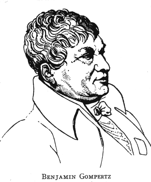
Benjamin Gompertz, the actuary who proposed the Gompertz law. Public domain, via Wikimedia Commons.

Benjamin Gompertz (1779–1865) was a largely self-taught mathematician and a London actuary. In a paper read to the Royal Society in 1825, he proposed that a person’s “power to oppose destruction” wears away so that, in equal small intervals of time, a person “lost equal portions of his remaining power to oppose destruction.”¹ If the mortality rate is inversely proportional to that power, it rises in geometric progression with age. Gompertz tested the idea against several life tables of his day and found that, over long stretches of adult life, the logarithms of the mortality rates did increase in nearly equal steps.¹ He also recognised that death has two co-existing causes, chance and “an increased inability to withstand destruction,” and that his formula described only the second.⁵¹

William Makeham supplied the first in 1860 by adding a constant term to the mortality rate, representing causes of death that do not depend on age.³ The resulting Gompertz–Makeham law dominated the graduation (smoothing) of actuarial tables for the next century.

Whole-life and logistic formulae

The Danish astronomer and actuary Thorvald Thiele published the first formula for the whole of life in 1871. It sums three terms: a declining exponential for childhood, a bell-shaped hump for early adulthood, and a Gompertz exponential for old age.²¹ Wilfred Perks introduced logistic formulae in 1932, in which the exponential rise flattens at the oldest ages.¹⁶ In 1959 Robert Beard showed how such flattening could arise. Suppose individuals differ in frailty, and each individual’s Gompertz mortality rate is multiplied by it. The frailest die first, and if frailty follows a gamma distribution the mortality rate of the surviving population takes a logistic form.¹⁸

Reliability, frailty and multi-component models

Waloddi Weibull, a Swedish engineer studying the strength and fatigue of materials, published the distribution that bears his name in 1939 and popularised it in English in 1951.⁵²⁵³ In it the failure rate rises as a power of age rather than exponentially, and it became the standard model of failure in reliability engineering before biologists applied it to organisms.¹⁵

In 1960 Bernard Strehler and Albert Mildvan proposed the first mechanistic theory of the Gompertz law (described above).²⁵ In 1979 James Vaupel, Kenneth Manton and Eric Stallard formalised frailty as a random multiplier of each individual’s mortality rate and showed how it bends the population curve.¹⁷ In the same year the ecologist William Siler proposed a five-parameter competing-risk model for animal populations,²² and in 1980 Heligman and Pollard published an eight-parameter model that captured the young-adult hump in human data.²³

Forecasting and the plateau debate

Ronald Lee and Lawrence Carter’s 1992 model shifted attention from the age pattern of mortality to its trend over calendar time.¹⁰ In the same issue of Science that year, two studies of very large insect cohorts reported that mortality rates stop rising at advanced ages, contrary to the Gompertz law:⁴⁵ James Carey and colleagues followed 1.2 million Mediterranean fruit flies, and James Curtsinger and colleagues followed Drosophila. Väinö Kannisto, Roger Thatcher and Vaupel then showed that the human mortality rate above age 80 is better described by a logistic curve than by an exponential.¹⁹ The question of whether human mortality reaches a true plateau has been argued since, with large studies on both sides.⁶⁷⁸

Data and figures

Figures 1 to 8 were drawn for this article from the Social Security Administration’s Period Life Table, 2023, as used in the 2026 Trustees Report. Mortality rates were computed from the table’s chance of dying within the year as $μ = - ln (1 - q_{x})$ , and deaths at each age as the share still alive times the mortality rate. Figures 6 and 8 pass through the observed rates at ages 75 and 95, and the Weibull curve in Figure 5 through the rate at 70; the other fitted curves minimise squared error in log mortality rate. The typical miss in the comparison table is the root-mean-square error on the log scale, converted to a percentage, $e^{RMSE} - 1$ . The portrait of Gompertz is in the public domain (Wikimedia Commons).

Gompertz B (1825). “On the nature of the function expressive of the law of human mortality, and on a new mode of determining the value of life contingencies”. Philosophical Transactions of the Royal Society of London. 115: 513–583. doi:10.1098/rstl.1825.0026 ↩↩² ↩³ ↩⁴
Finch CE, Pike MC, Witten M (1990). “Slow mortality rate accelerations during aging in some animals approximate that of humans”. Science. 249 (4971): 902–905. doi:10.1126/science.2392680 ↩↩² ↩³ ↩⁴
Makeham WM (1860). “On the law of mortality and the construction of annuity tables”. The Assurance Magazine, and Journal of the Institute of Actuaries. 8 (6): 301–310. doi:10.1017/S204616580000126X ↩↩² ↩³
Carey JR, Liedo P, Orozco D, Vaupel JW (1992). “Slowing of mortality rates at older ages in large medfly cohorts”. Science. 258 (5081): 457–461. doi:10.1126/science.1411540 ↩↩² ↩³ ↩⁴
Curtsinger JW, Fukui HH, Townsend DR, Vaupel JW (1992). “Demography of genotypes: failure of the limited life-span paradigm in Drosophila melanogaster”. Science. 258 (5081): 461–463. doi:10.1126/science.1411541 ↩↩² ↩³
Barbi E, Lagona F, Marsili M, Vaupel JW, Wachter KW (2018). “The plateau of human mortality: Demography of longevity pioneers”. Science. 360 (6396): 1459–1461. doi:10.1126/science.aat3119 ↩↩² ↩³ ↩⁴
Newman SJ (2018). “Errors as a primary cause of late-life mortality deceleration and plateaus”. PLOS Biology. 16 (12): e2006776. doi:10.1371/journal.pbio.2006776 ↩↩² ↩³ ↩⁴
Gavrilov LA, Gavrilova NS (2011). “Mortality measurement at advanced ages: a study of the Social Security Administration Death Master File”. North American Actuarial Journal. 15 (3): 432–447. doi:10.1080/10920277.2011.10597629 ↩↩² ↩³ ↩⁴ ↩⁵ ↩⁶
Jones OR, Scheuerlein A, Salguero-Gómez R, Camarda CG, Schaible R, et al. (2014). “Diversity of ageing across the tree of life”. Nature. 505 (7482): 169–173. doi:10.1038/nature12789 ↩↩² ↩³ ↩⁴ ↩⁵
Lee RD, Carter LR (1992). “Modeling and forecasting U.S. mortality”. Journal of the American Statistical Association. 87 (419): 659–671. doi:10.1080/01621459.1992.10475265 ↩↩² ↩³ ↩⁴
de Moivre A (1725). Annuities upon Lives. London. Digitised copy ↩↩²
Missov TI, Lenart A, Nemeth L, Canudas-Romo V, Vaupel JW (2015). “The Gompertz force of mortality in terms of the modal age at death”. Demographic Research. 32 (36): 1031–1048. doi:10.4054/DemRes.2015.32.36 ↩↩²
Horiuchi S, Wilmoth JR (1998). “Deceleration in the age pattern of mortality at older ages”. Demography. 35 (4): 391–412. doi:10.2307/3004009 ↩↩² ↩³
Juckett DA, Rosenberg B (1993). “Comparison of the Gompertz and Weibull functions as descriptors for human mortality distributions and their intersections”. Mechanisms of Ageing and Development. 69 (1–2): 1–31. doi:10.1016/0047-6374(93)90068-3 ↩↩² ↩³
Ricklefs RE, Scheuerlein A (2002). “Biological implications of the Weibull and Gompertz models of aging”. The Journals of Gerontology Series A. 57 (2): B69–B76. doi:10.1093/gerona/57.2.B69 ↩↩² ↩³
Perks W (1932). “On some experiments in the graduation of mortality statistics”. Journal of the Institute of Actuaries. 63 (1): 12–57. doi:10.1017/S0020268100046680 ↩↩²
Vaupel JW, Manton KG, Stallard E (1979). “The impact of heterogeneity in individual frailty on the dynamics of mortality”. Demography. 16 (3): 439–454. doi:10.2307/2061224 ↩↩² ↩³
Beard RE (1959). “Note on some mathematical mortality models”. In Wolstenholme GEW, O’Connor M (eds.), The Lifespan of Animals. CIBA Foundation Colloquia on Ageing, vol. 5. pp. 302–311. doi:10.1002/9780470715253.app1 ↩↩² ↩³ ↩⁴
Thatcher AR, Kannisto V, Vaupel JW (1998). The Force of Mortality at Ages 80 to 120. Odense Monographs on Population Aging 5. Odense University Press. ISBN 87-7838-381-1. Full text ↩↩² ↩³ ↩⁴
Wilmoth JR, Andreev K, Jdanov D, Glei DA, Riffe T, et al. (2025). Methods Protocol for the Human Mortality Database, version 6. PDF ↩↩² ↩³
Thiele TN (1871). “On a mathematical formula to express the rate of mortality throughout the whole of life, tested by a series of observations made use of by the Danish Life Insurance Company of 1871”. Journal of the Institute of Actuaries and Assurance Magazine. 16 (5): 313–329. doi:10.1017/S2046167400043688 ↩↩²
Siler W (1979). “A competing-risk model for animal mortality”. Ecology. 60 (4): 750–757. doi:10.2307/1936612 ↩↩²
Heligman L, Pollard JH (1980). “The age pattern of mortality”. Journal of the Institute of Actuaries. 107 (1): 49–80. doi:10.1017/S0020268100040257 ↩↩²
Weon BM, Je JH (2009). “Theoretical estimation of maximum human lifespan”. Biogerontology. 10 (1): 65–71. doi:10.1007/s10522-008-9156-4 ↩↩²
Strehler BL, Mildvan AS (1960). “General theory of mortality and aging”. Science. 132 (3418): 14–21. doi:10.1126/science.132.3418.14 ↩↩²
Gavrilov LA, Gavrilova NS (2001). “The reliability theory of aging and longevity”. Journal of Theoretical Biology. 213 (4): 527–545. doi:10.1006/jtbi.2001.2430 ↩↩² ↩³
Medawar PB (1952). An Unsolved Problem of Biology. London: H. K. Lewis. ↩
Hamilton WD (1966). “The moulding of senescence by natural selection”. Journal of Theoretical Biology. 12 (1): 12–45. doi:10.1016/0022-5193(66)90184-6 ↩
Karin O, Agrawal A, Porat Z, Krizhanovsky V, Alon U (2019). “Senescent cell turnover slows with age providing an explanation for the Gompertz law”. Nature Communications. 10: 5495. doi:10.1038/s41467-019-13192-4 ↩
Stroustrup N, Anthony WE, Nash ZM, Gowda V, Gomez A, et al. (2016). “The temporal scaling of Caenorhabditis elegans ageing”. Nature. 530 (7588): 103–107. doi:10.1038/nature16550 ↩↩²
Vaupel JW, Carey JR, Christensen K, Johnson TE, Yashin AI, et al. (1998). “Biodemographic trajectories of longevity”. Science. 280 (5365): 855–860. doi:10.1126/science.280.5365.855 ↩
Gampe J (2010). “Human mortality beyond age 110”. In Maier H, Gampe J, Jeune B, Robine J-M, Vaupel JW (eds.), Supercentenarians. Demographic Research Monographs 7. Springer. pp. 219–230. doi:10.1007/978-3-642-11520-2_13 ↩
Dong X, Milholland B, Vijg J (2016). “Evidence for a limit to human lifespan”. Nature. 538 (7624): 257–259. doi:10.1038/nature19793 ↩
Lenart A, Vaupel JW (2017). “Questionable evidence for a limit to human lifespan”. Nature. 546 (7660): E13–E14. doi:10.1038/nature22790 ↩
Ruby JG, Smith M, Buffenstein R (2018). “Naked mole-rat mortality rates defy Gompertzian laws by not increasing with age”. eLife. 7: e31157. doi:10.7554/eLife.31157 ↩
Brouhns N, Denuit M, Vermunt JK (2002). “A Poisson log-bilinear regression approach to the construction of projected lifetables”. Insurance: Mathematics and Economics. 31 (3): 373–393. doi:10.1016/S0167-6687(02)00185-3 ↩
Li N, Lee R (2005). “Coherent mortality forecasts for a group of populations: an extension of the Lee–Carter method”. Demography. 42 (3): 575–594. doi:10.1353/dem.2005.0021 ↩
Renshaw AE, Haberman S (2006). “A cohort-based extension to the Lee–Carter model for mortality reduction factors”. Insurance: Mathematics and Economics. 38 (3): 556–570. doi:10.1016/j.insmatheco.2005.12.001 ↩
Cairns AJG, Blake D, Dowd K (2006). “A two-factor model for stochastic mortality with parameter uncertainty: theory and calibration”. Journal of Risk and Insurance. 73 (4): 687–718. doi:10.1111/j.1539-6975.2006.00195.x ↩↩²
Currie ID, Durban M, Eilers PHC (2004). “Smoothing and forecasting mortality rates”. Statistical Modelling. 4 (4): 279–298. doi:10.1191/1471082X04st080oa ↩
Brass W (1971). “On the scale of mortality”. In Brass W (ed.), Biological Aspects of Demography. London: Taylor & Francis. pp. 69–110. ↩↩²
Coale AJ, Demeny P (1966). Regional Model Life Tables and Stable Populations. Princeton: Princeton University Press. ↩
Wilmoth JR (2000). “Demography of longevity: past, present, and future trends”. Experimental Gerontology. 35 (9–10): 1111–1129. doi:10.1016/S0531-5565(00)00194-7 ↩
Vaupel JW (2010). “Biodemography of human ageing”. Nature. 464 (7288): 536–542. doi:10.1038/nature08984 ↩
Pletcher SD (1999). “Model fitting and hypothesis testing for age-specific mortality data”. Journal of Evolutionary Biology. 12 (3): 430–439. doi:10.1046/j.1420-9101.1999.00058.x ↩↩² ↩³
Colchero F, Jones OR, Rebke M (2012). “BaSTA: an R package for Bayesian estimation of age-specific survival from incomplete mark–recapture/recovery data with covariates”. Methods in Ecology and Evolution. 3 (3): 466–470. doi:10.1111/j.2041-210X.2012.00186.x ↩↩²
Tai TH, Noymer A (2018). “Models for estimating empirical Gompertz mortality: with an application to evolution of the Gompertzian slope”. Population Ecology. 60 (1–2): 171–184. doi:10.1007/s10144-018-0609-6 ↩
Mair W, Goymer P, Pletcher SD, Partridge L (2003). “Demography of dietary restriction and death in Drosophila”. Science. 301 (5640): 1731–1733. doi:10.1126/science.1086016 ↩
Graunt J (1662). Natural and Political Observations Mentioned in a Following Index, and Made upon the Bills of Mortality. London. Digitised copy ↩
Halley E (1693). “An estimate of the degrees of the mortality of mankind, drawn from curious tables of the births and funerals at the city of Breslaw; with an attempt to ascertain the price of annuities upon lives”. Philosophical Transactions. 17 (196): 596–610. doi:10.1098/rstl.1693.0007 ↩
Kirkwood TBL (2015). “Deciphering death: a commentary on Gompertz (1825) ‘On the nature of the function expressive of the law of human mortality, and on a new mode of determining the value of life contingencies’”. Philosophical Transactions of the Royal Society B. 370 (1666): 20140379. doi:10.1098/rstb.2014.0379 ↩
Weibull W (1939). “A statistical theory of the strength of materials”. Ingeniörsvetenskapsakademiens Handlingar. 151. Stockholm. ↩
Weibull W (1951). “A statistical distribution function of wide applicability”. Journal of Applied Mechanics. 18 (3): 293–297. doi:10.1115/1.4010337 ↩

Brinedew

Mortality rate models

Terminology

The age pattern of human mortality

Models of the age pattern

De Moivre’s law

Gompertz law

Gompertz–Makeham law

Weibull model

Logistic models

Multi-component models

Weon–Je model

Comparison

Explanations of the Gompertz law

Strehler–Mildvan theory

Reliability theory

Heterogeneity and selection

Evolutionary theory

Cellular and physiological models

Late-life deceleration and the plateau debate

Evidence from other species

Evidence in humans

Mortality across species

Changes over time and forecasting

Lee–Carter and its extensions

Relational models

Rectangularisation and the shifting mode

Estimation

Data and likelihood

Practical difficulties

Applications

History

Life tables before models

Gompertz and Makeham

Whole-life and logistic formulae

Reliability, frailty and multi-component models

Forecasting and the plateau debate

Data and figures

Table of Contents

Brinedew

Mortality rate models

Terminology

The age pattern of human mortality

Models of the age pattern

De Moivre’s law

Gompertz law

Gompertz–Makeham law

Weibull model

Logistic models

Multi-component models

Weon–Je model

Comparison

Explanations of the Gompertz law

Strehler–Mildvan theory

Reliability theory

Heterogeneity and selection

Evolutionary theory

Cellular and physiological models

Late-life deceleration and the plateau debate

Evidence from other species

Evidence in humans

Mortality across species

Changes over time and forecasting

Lee–Carter and its extensions

Relational models

Rectangularisation and the shifting mode

Estimation

Data and likelihood

Practical difficulties

Applications

History

Life tables before models

Gompertz and Makeham

Whole-life and logistic formulae

Reliability, frailty and multi-component models

Forecasting and the plateau debate

Data and figures

Footnotes

Table of Contents